3.1 Modeling and understanding the statistics of weekly averages
The principal mechanism of tropical-extratropical interaction is through diabatically forced Rossby waves. On seasonal and longer scales, tropical diabatic heating is strongly linked to tropical SST; hence one speaks of an "SST-forced" global response as in Chapter 2. On the subseasonal scales of interest here, the SST variability is relatively weak, and its coupling to the heating variability is much less rigid. The heating variability itself is considerable, however, and has a significant extratropical impact. Some of this variability (especially that associated with the MJO) is predictable, and raises the hope that at least some aspects of subseasonal extratropical variability may therefore also be predictable. Unfortunately, for various reasons the simulation and predictability of subseasonal tropical heating variations has thus far proved difficult in general circulation models. This has been a major stumbling block in capitalizing on this source of subseasonal extratropical predictability.
Inspired by the success in Figs 2.1-2.4 of simple empirical predictions of seasonal tropical SST variations and their global impact, we have recently constructed a linear inverse model (LIM) suitable for studies of atmospheric variability and predictability on weekly time scales using global observations of the past 30 years. Notably, it includes tropical diabatic heating as an evolving model variable rather than as an externally specified forcing. It also includes, in effect, the feedback of the extratropical weather systems on the more slowly varying circulation. We have found both of these features to be important contributors to the model's realism.
The model is concerned with the behavior of 7-day running mean
anomalies of extratropical streamfunction and column-averaged tropical
diabatic heating. It assumes that atmospheric states separated by time
lags  are related as
x(t+
 ) = G(
 ) x(t) +
  , where G is a linear
operator and
  is
noise. This implies that the zero-lag and time-lag-covariance matrices
of x are related as C(
 ) = G(
 )C(0). We use this relationship at a particular lag,
say
  = 5 days, to obtain
G(5) from observational estimates of C(5) and
C(0). We then make another assumption that is at the heart of
the LIM formalism, that distinguishes it from other empirical models,
and that enables one to make dynamically meaningful diagnoses of
direct relevance to modelers. This is that G(
 ) satisfies the relation
G(
 ) = exp(L
 ), where L is a constant
linear operator. We use this to obtain L from G(5), and
having done so, use it again to obtain G for all other lags. We
are finally in a position to make forecasts for all lags as
x(t+
 ) = G(
 ) x(t). Crucially, having
obtained L, we can also diagnose the relative importance of its
elements associated with tropical-extratropical and internal
extratropical interactions. For example, we can use L to
estimate what the statistics of extratropical variability would be
without diabatic forcing from the tropics.
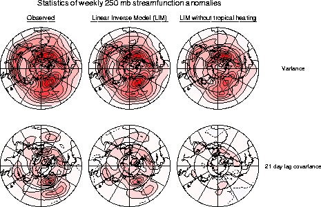
Figure 3.1 demonstrates the success of this model in reproducing the observed variance and 21-day lag covariance of 7-day running-mean anomalies of 250 mb streamfunction during northern winter. Note again that we are effectively using the observed 5-day lag covariances to predict the 21-day lag covariances here. The comparison of the observed and predicted covariances is clearly encouraging. The right column shows that the effect of tropical heating is relatively small on the variance but relatively large on the 21-day lag covariance. This is consistent with our finding that although tropical heating contributes a relatively small portion of the extratropical variability, it contributes a large portion of the predictable variability.

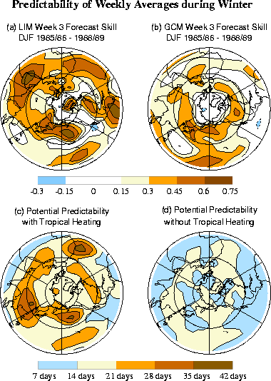
Forecast skill is an important test of any model. The LIM is better at forecasting Week 2 anomalies than a dynamical model based on the linearized baroclinic equations of motion (with many more than the LIM's 37 degrees of freedom) that is forced with observed tropical heating throughout the forecast. Indeed at Week 2 the LIM's skill is competitive with NCEP's MRF model with nominally O(106) degrees of freedom. The upper panel of Fig. 3.2 shows such a comparison of Week 3 forecast skill during the winters of 1985/86-1988/89. Other experiments show that this encouraging forecast performance is not limited to years of El Niño or La Niña episodes.

The LIM assumes that the dynamics of extratropical low-frequency variability are linear, stable, and stochastically forced. The approximate validity of these assumptions has been demonstrated through several tests. A potentially limiting aspect of such a stable linear model with decaying eigenmodes concerns its ability to predict anomaly growth. We have nevertheless found, through a singular vector analysis of the model's propagator G, that predictable anomaly growth can and does occur in this dynamical system through constructive modal interference. Examination of the initial structures associated with optimal anomaly growth further confirms the importance of tropical heating anomalies associated with El Niño and La Niña as well as Madden-Julian oscillation episodes in the predictable dynamics of the extratropical circulation.
The LIM formalism also allows one to estimate predictability limits in a straightforward manner. Indeed it allows one to estimate the expected skill of any individual forecast from the strength of its predicted signal. Given that in many cases the predictable signal is associated with tropical forcing, one can quantify the effect of that forcing on extratropical predictability. Our general conclusion is that without tropical forcing, extratropical weekly averages may be predictable only about two weeks ahead, but with tropical forcing, they may be predictable as far as seven weeks ahead. This difference is highlighted in the lower panel of Fig. 3.2. This suggests that accurate prediction of tropical diabatic heating, rather than of tropical sea surface temperatures per se, is key to enhancing extratropical predictability on these time scales.
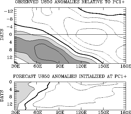
As mentioned earlier, most current GCMs have difficulty in representing and predicting heating variations on these scales. This is especially true of the NCEP MRF model. We have documented significant deficiencies in the "reanalysis version" of that model in maintaining and propagating MJO-related heating and circulation anomalies. Figure 3.3 shows that forecasts initialized when the MJO is active over the Indian ocean are unable to represent the subsequent eastward propagation of 850-mb zonal wind anomalies; indeed they do not predict propagation at all but a rapid decay. This has been demonstrated to have a negative impact on extratropical forecasts.

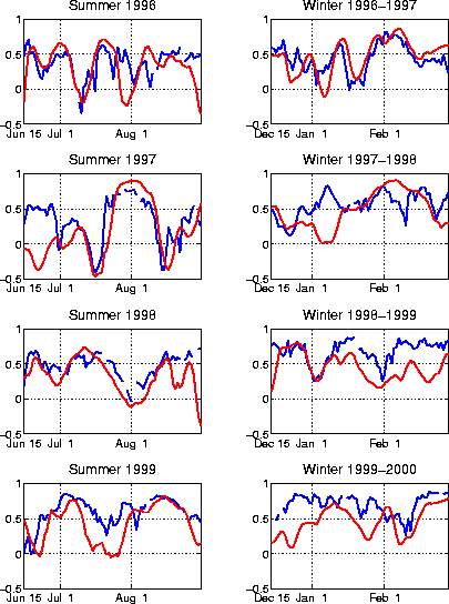
Figure 3.4 shows that the LIM's forecast skill over the PNA region is comparable to that of the operational MRF ensemble mean, especially in summer. The MRF can represent some phenomena that the LIM cannot, such as nonlinear baroclinic cyclogenesis and blocking. To the extent that these phenomena are predictable, the MRF should have an advantage. This is indeed the case in Week 1. By Week 2, these phenomena become unpredictable; even so, their role in exciting larger scale, slowly evolving structures such as the PNA pattern in Week 1 can contribute to maintaining forecast skill in Week 2. On the other hand, the LIM is much better at predicting subseasonal variations of tropical convection than the MRF, and being an anomaly model, also does not suffer from climate drift by construction. Therefore, it seems likely that the comparable skill of the LIM and the operational MRF models is not arising entirely from the same sources. This is in contrast to the seasonal prediction problem discussed in Chapter 2, in which the comparable skill of GCMs and simple statistical models arises from essentially the same source. To the extent that the sources of Week 2 forecast skill in the statistical and dynamical models are distinct, combining the two forecasts should, in principle, yield forecasts that are superior to either in isolation. Constructing such a combination is currently one of our main priorities.
