3.4 The relationship between spread and skill in the operational NCEP ensemble forecasts
The studies discussed in sections 3.1 and 3.2 show that statistical models can have skill comparable to NWP models in the Week 2 to Week 3 range because subseasonal variations of tropical convection, which the NWP models do not simulate well, provide significant predictive information. However, the NWP models, unlike the statistical models, can provide information on day-to-day variations of both the signal (the amplitude of the predictable component of the forecast) and noise (the amplitude of the unpredictable component of the forecast). The statistical models assume the noise to be stationary, i.e. to not vary from forecast to forecast. An NWP ensemble can be used to estimate the noise in each forecast case, and hence a case-dependent estimate of the RMS error of the ensemble-mean forecast.
The simplest measure of forecast noise is the width, or spread, of the forecast probability distribution for any quantity of interest. CDC scientists have investigated the relationship between spread and skill in the operational NCEP forecast ensembles using an archive of operational forecasts maintained at CDC since 1995. Simple statistical considerations show that such a measure is most useful when the case-to-case variability of the ensemble spread is large. This was shown to be true in two winters of operational ensemble predictions. However, the short data record precluded a detailed analysis of the dynamical mechanisms of the spread variability.
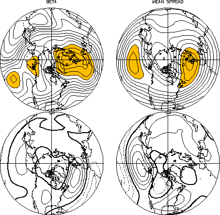
To get around this limitation, a five-level linear quasi-geostrophic (QG) model, linearized about three-day segments of the observed flow for 21 years, was used to model the spread variability. The fundamental assumption was that day-to-day variations of spread are due primarily to day-to-day variations in the growth rate of small perturbations during the forecast period, and that day-to-day variations in the initial error, i.e. in the spread of the analysis-error distribution, are either unimportant or not well sampled. The five-level model was able to reproduce the main results (not shown) of the shorter 2-winter study mentioned above. When run for 21 years, the QG model showed the largest spread variability of 3-day forecasts over the eastern Pacific and eastern Atlantic oceans, which was associated with modulations of the local jets by the PNA and NAO modes of low-frequency variability (Fig. 3.10). To the extent that such modulations are predictable, the results from this study suggest that skill should also be most predicable in these regions.

 ), estimated
from 3-day integrations of the five-level linear QG model. S is
normalized by the mean amplitude of the initial perturbations used in
the ensemble integrations. Contour interval for
  is 0.01, with values
greater than
0.28 shaded. Contour interval for normalized S is 0.25, with values
greater than 4 shaded. Lower Panels: Map of correlations between
time series of lnS at points indicated by the black rectangles and
three-day averaged 300 hPa streamfunction. Contour interval is
0.1, negative values are dashed, and the zero line is thick solid.