
NOAA Earth System Research Laboratory, R/GMD, 325 Broadway, Boulder, CO 80305-3328
Robert.Stone, Science and Technology Corporation, Boulder, CO
Updated April 2017
ACKNOWLEDGEMENTS: This study was supported by NOAA's Earth System Research Laboratory's (ESRL) Global Monitoring Division (GMD). Original content can be found at: Western Arctic Climate Change. This update includes ancillary analyses provided by D. Douglas (USGS) - sea ice conditions and regional phenology. The paper of Cox et al. (2017) provides the basis for the following presentation and many of the figures. C. Cox was supported by the Arctic Research Program (ARP) of the NOAA Climate Program Office (CPO). We also acknowledge the NCEP/NCAR Reanalysis Project: NCEP Reanalysis data were provided by NOAA/OAR/ESRL PSD, Boulder, Colorado, USA, Website at: http://www.esrl.noaa.gov/psd/.
The Arctic is especially prone to warming in response to globally increasing concentrations of greenhouse gases through a mechanism referred to as "Arctic Amplification" (e.g., Serreze et al., 2009 and references therein). There is convincing evidence of both climate and environmental changes across the Alaskan Arctic and northern Siberia. The cause and effect of Arctic climate change is of great interest across disciplines. To what degree changes are due to anthropogenic influences or natural variations has not been determined. Using assimilated data from a network of observatories around the Arctic, teams are studying aspects of the mechanisms underlying observed changes (e.g., Uttal et al., 2016; Starkweather and Uttal, 2016). The NOAA/GML Barrow Observatory (BRW) is one of these sites where a long, comprehensive set of data has been collected. Following is an overview of changes in climate observed for the Pacific Arctic documenting trends in temperature, phenology and adjacent sea ice distributions, with a focus on BRW, which has been shown to be regionally representative. Some material and figures are adapted from Cox et al. (2017).
Note: Background and original content can be found at: Western Arctic Climate Change
Figure 1 is a composite set of maps that indicates dates when, on average, greening of tundra vegetation begins and ends each year and also the dates when sea ice begins to melt in spring and refreezes in autumn (see color scales). The ‘start of season’ and ‘end of season’ are referred to as SOS and EOS, respectively. The metric used to determine greening of vegetation is the Normalized Difference Vegetation Index (NDVI), and for sea ice melt and freeze signatures derived from microwave radiometry. Both measurements are derived from data collected by Polar orbiting satellites. Results are shown for SOS (a) and (b) and EOS (d) and (e), for years 1982-1999 (a and d) and 2000-2014 (b and e), respectively. In addition, the maps show the median boundary of the ice edge (bold white lines) as of June 1 and October 1 for the respective periods. At right, (c) and (f) compare SOS and EOS, by day of year (DOY), for 1982-1999 (blue trace) with 2000-2014 (red trace) along a latitudinal transect shown in (a).
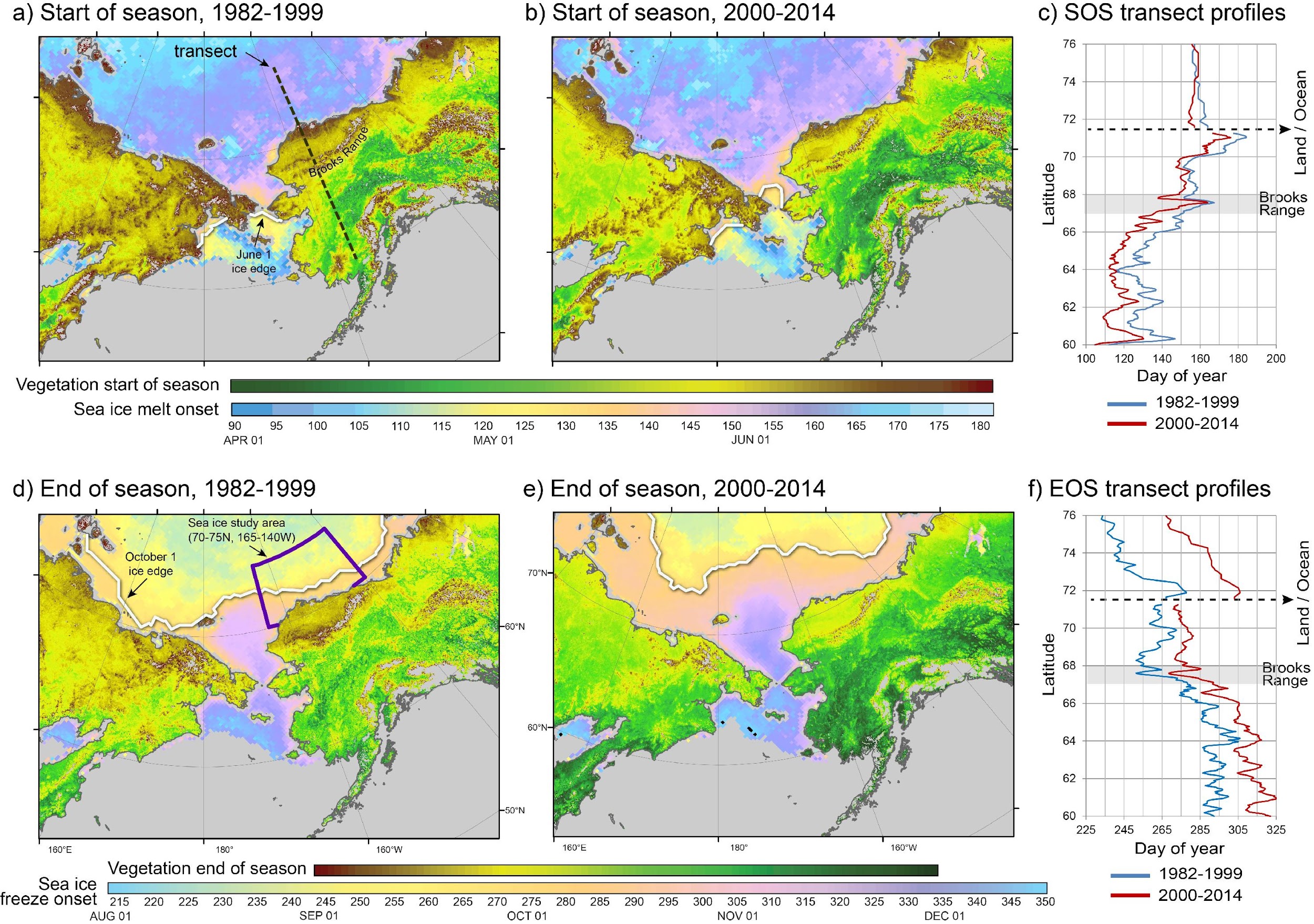
Cox et al. (2017) document how earlier snowmelt in spring and a longer growing season observed at BRW represent changes that are taking place across the Pacific Arctic (see: Barrow's Annual Snow Cycle; Ecological Responses to a Lengthening Snow-free Season for background and overview). Both earlier melt and later freeze, accompanied by unprecedented losses in summer sea ice, have contributed significantly to lengthening the snow-free period of the region as is manifested in Figure 1 via a comparison of the pre- and post-2000 periods.
The onset of the Arctic growing season is primarily constrained by surface air temperature, coupled to the same mechanisms that influence the timing of snowmelt. We find that shifts toward both earlier start dates and later end dates underlie the longer growing season. The earlier melt and green-up trends in the Pacific Arctic are primarily driven by rising air temperatures that in turn are associated with regional circulation patterns that favor advection of warm air from the North Pacific during late winter or early spring (Stone et al., 2005; Cox et al., 2017). EOS trends in Pacific Arctic phenology are, on the other hand, linked to the distribution of sea ice and timing of ice formation because on-land flow from the adjacent seas influence the timing of freeze as well as accumulation of snow in autumn. During the period 1982-1999, sea ice formation in the region north of BRW, highlighted in Figure 1d, occurred roughly at the same time the growing season ended, but since 2000 has occurred, on average, later by several weeks (Figure 1f). Greater solar heating of the open ocean water during summer and delayed ice formation in autumn underlies the persistent rise in October and November air temperatures at BRW, as discussed below.
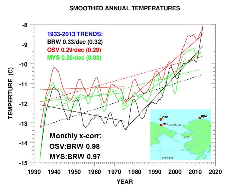
The seven-year smoothed time series reveal the multiyear variability of the regional temperature regime. Linear regressions were performed (on the actual monthly averages) for the period of overlap, 1933-2014 (dashed), and also periods 1933-1975 and 1976-2014 (solid). Regionally, the rise in temperature over the entire period has been about 0.3°C ±0.3 at the 95% confidence level as the upper left legend indicates. However, until the mid 1970s, slight regional cooling is indicated, followed by a dramatic increase beginning around 1976. The annual temperature of the region has risen by about 1°C/decade since the mid 1970s. The warming occurs subsequent to a well-documented shift in circulation patterns affecting the North Pacific around 1976 (Hare and Mantua, 2000). At that time, the Aleutian Low pressure system intensified resulting in increased cyclonic activity that favored the advection of warm, moist air into the Pacific Arctic. Warm-air advection combined with radiative warming by clouds likely contributes to rising temperature trends (Stone, 1997; Stone et al., 2005). The three stations show remarkably similar variations and trends over a long period of time, suggesting that the underlying mechanism of change is related to changes in atmospheric circulation on a synoptic scale. The cross-correlation between the two Russian sites and BRW are indicated in the lower, left legends of Figure 2.
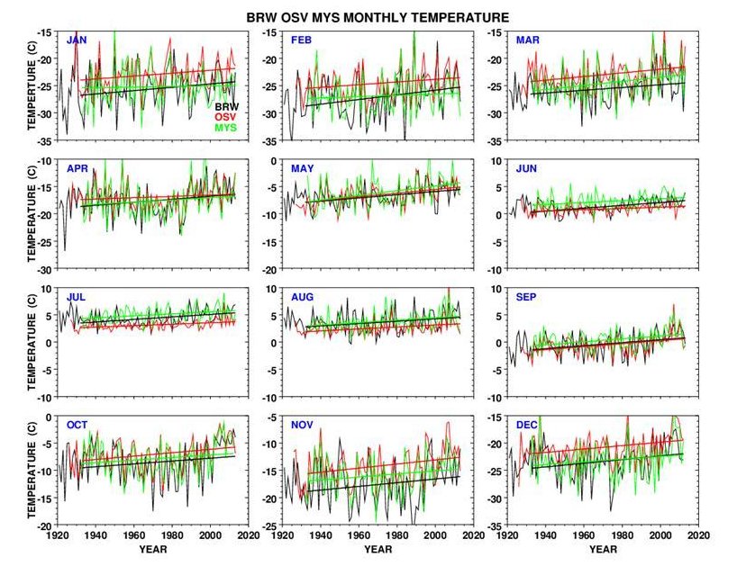
Figure 3 is a multiple plot showing time series for BRW, OSV and MYS (color-coded), by month; again fitted linearly to show trends. Note that OVV tends to be warmer than BRW by as much as 5°C in winter months but is slightly cooler mid summer. This is probably due to the influence of open water, but overall the cross correlations are very high as shown in Figure 2. There have been significant increases in temperature for all months and especially in autumn and winter, with most of the rise occurring since the mid 1970s.
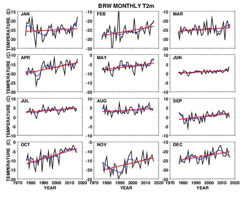
An analysis of the BRW monthly mean temperatures for 1975-2016 is presented in Figure 4. In this case, the red lines are linear fits and blue traces show seven-year smoothed data that reveal periods of cooling as well as warming. Again, overall warming is indicated for all months but we find that the most dramatic warming has occurred during autumn. This is particularly true for October and since the late 1990s, with similar enhancements extending through December. However, there appears to be some leveling off in the most recent years. The main reason for the post-2000 increase in autumn temperatures at BRW is attributed to delayed sea ice formation in the Chukchi and Beaufort Sea region; the delay, in turn, due to declining summer sea ice as explained by Cox et al. (2017).
Impacts stemming from declining Arctic sea ice include a lengthening of the snow-free season that affects terrestrial phenology (Figure 1), permafrost, biogeochemical cycles, as well as bird and wildlife habitats. These are discussed at: Barrow's Annual Snow Cycle; Ecological Responses to a Lengthening Snow-free Season and by Cox et al. 2017; references therein. In addition, the surface-atmosphere radiation balance is undergoing changes (see: Barrow Radiation Climatology). Although fitted linearly, it is obvious that none of these metrics show monotonic trends. Year-to-year variations are large and multi-year variations are evident when time series are smoothed. Clearly, the drivers of change are not solely related to global warming due to greenhouse gas concentrations that are increasing more monotonic. Natural variations have always been large in the Arctic, preventing a strict partitioning of anthropogenic versus natural influences. A major, and apparently natural, underlying mechanism for change relates to atmospheric circulation patterns, as in the case of the mid 1970s shift affecting the North Pacific mentioned above. Following is a discussion of how synoptic-scale circulation patterns, south and north of Alaska, influence the climate and ecology of the Pacific Arctic region.
Atmospheric circulation patterns strongly influence the timing of snowmelt (Stone et al., 2002), vegetation green-up and onset of sea ice melt (Stone et al., 2005; Cox et al., 2017). At BRW, years with late snowmelt are associated with the presence of a high-pressure system north of Alaska, the Beaufort Sea Anticyclone (BSA). If present during spring, the BSA tends to block northward flow of warmer air circulating around the Aleutian Low (AL). This is illustrated in Figure 5 (left panel), which shows how the BSA is coupled with the AL to form a N-S dipole. Such a pattern keeps northern regions cold and relatively dry and snow cover remains more extensive as evidenced in Fig. 5 by the NDVI shading.
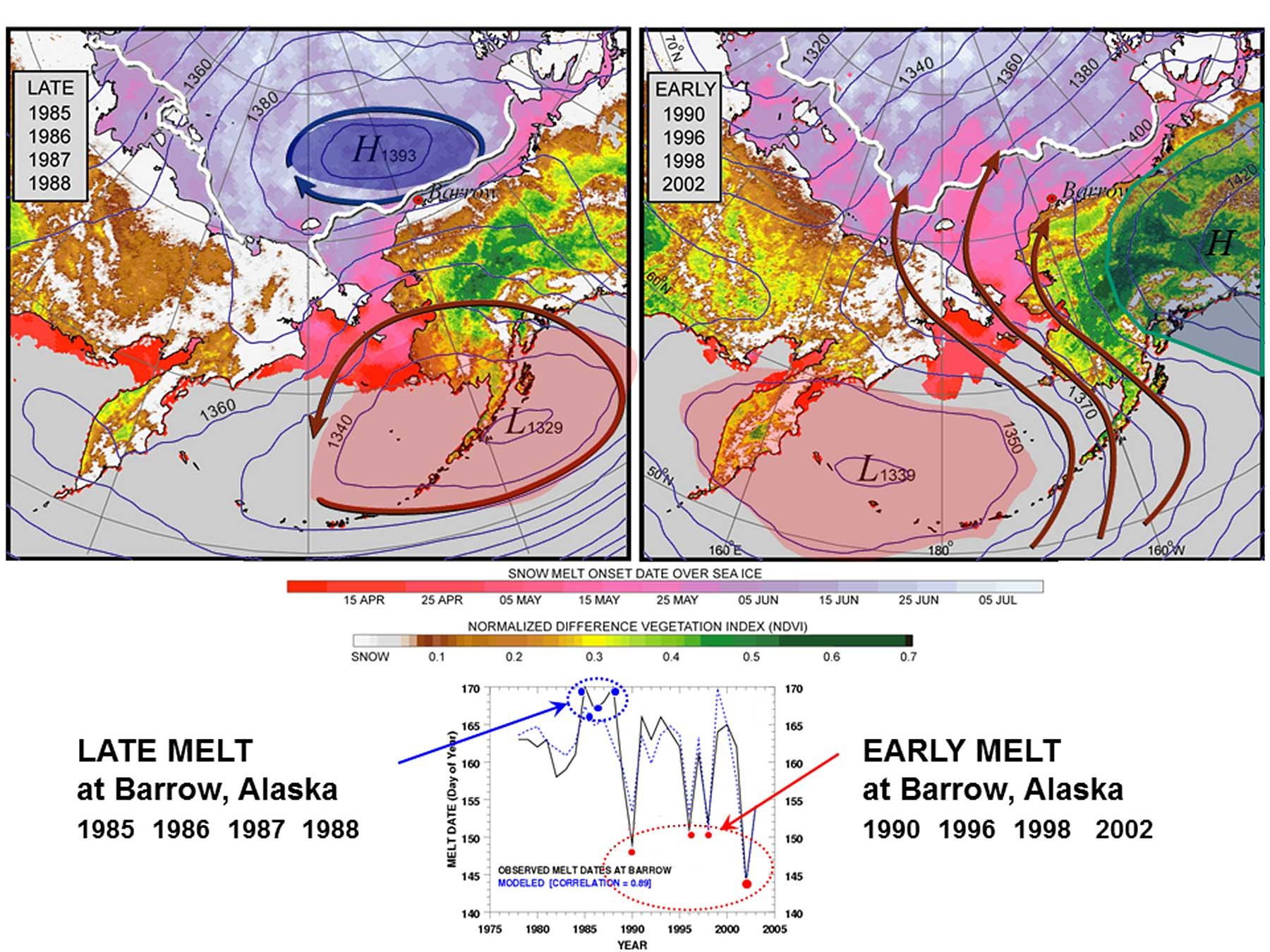
In contrast, years with early snowmelt are associated with a westward shift of the AL that establishes an east-to-west dipole with a high-pressure ridge having its axis extend into Alaska (Figure 5 (right panel)). This pattern favors the advection of warm Pacific air into the Arctic, shown schematically by red arrows. Similar analysis (below; Figure 8) show how this particular pattern persisted during May 2015 and May 2016, resulting in heat waves across the North Slope of Alaska.
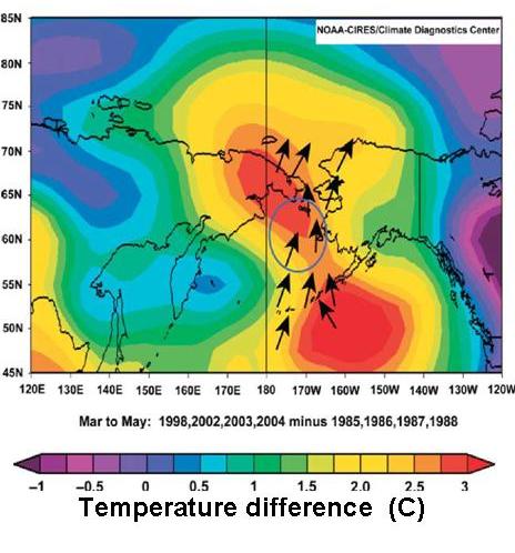
Years of extreme ice retreat typically align with earlier snowmelt and the onset of ice melt because warm Pacific air is transported through the Bering Straight and over adjacent lands. This is shown schematically in Figure 6 by differencing the temperature fields for four years of early snowmelt and four years of late snowmelt at BRW. Due to the much stronger E-W pressure gradient during years of early melt (Figure 5 (right)), warm Pacific air floods the Arctic Basin, accelerating snowmelt over terrestrial regions and promoting earlier onset of ice melt in the Chukchi/Beaufort region. An early, and thus prolonged, melt season leads to greater late-summer ice retreat (Stone et al., 2005).
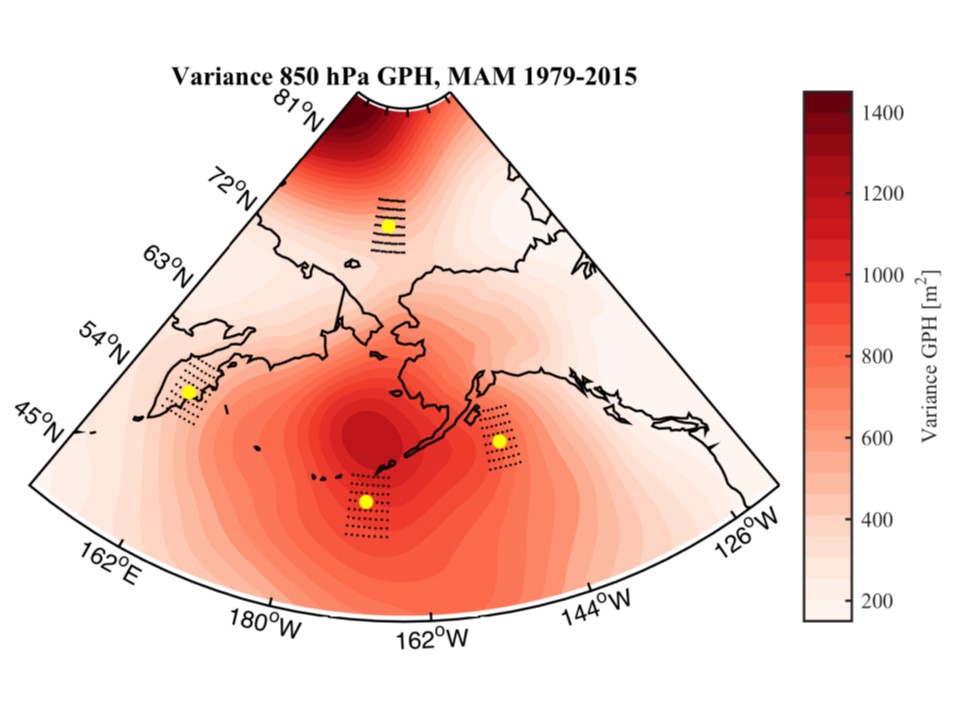
Prior analyses have demonstrated that atmospheric dynamics play a major role in determining the temperature regime and the timing of snow and ice melt in the Pacific Arctic region. Synoptic-scale influences were documented by Stone (1997) and further conceptualized using case studies presented in Stone et al. (2002) and Stone et al. (2005). Cox et al. (2017) examines more thoroughly the impact of the E-W dipole pattern described above, illustrated in Fig. 5 (right). On the basis of climatology and subsets of data associated with early and late years of snowmelt at BRW, a four-point matrix of points was selected to enable quantifying the north-south (N-S) and east-west (E-W) dipole patterns illustrated in Fig. 5. The approach was introduced at: Barrow's Annual Snow Cycle; Ecological Responses to a Lengthening Snow-free Season (Fig. 4 (g) and (h)), where an E-W index was derived as the difference between geopotential height at 850 hPa at 150°W and 160°E longitude along latitude 55°N. Here, N-S is similarly defined by differencing the geopotential heights at 75°N and 50°N latitude along longitude 170°W.
The selection of points is somewhat arbitrary, chosen on the basis of a number of case studies that distinguish conditions that either block or favor flow of Pacific air northward. Figure 7 shows the location of points, noting that evaluations were made for many points in the vicinity of each to determine sensitivity of the respective indices to position. The 850 hPa field has high variability in the region of the AL and thus it is its position and intensity that primarily determine the sign and magnitude of E-W and N-S indices. Once the matrix is defined, time series of these indices can be calculated from values of 850 hPa heights at the four locations, available through NCEP/NCAR Reanalysis website: https://www.esrl.noaa.gov/psd/cgi-bin/data/composites/printpage.pl.
Time series of the indices can then be evaluated for variations and trends and correlated with other metrics to determine physical relationships. For instance, the correlation of BRW snowmelt date with the E-W index was examined by Cox et al. (2017: Fig.6 g,h); see also: Barrow's Annual Snow Cycle; Ecological Responses to a Lengthening Snow-free Season (Fig. 4 (g) and (h)). BRW snowmelt date was found to correlate with May average values of E-W (r =0.53, p < 0.001), showing that the advection of Pacific air influences the timing of melt as well as May temperatures.
By combining E-W and N-S, a single index can be generated that captures the synoptic condition of the entire North Pacific-Pacific Arctic region, indicating potential for advection of warm air from the North Pacific into the Arctic. This index has been named ALBSA for the Aleutian Low and Beaufort Sea Anticyclone that are centers of action within the domain.
The ALBSA index is defined by differencing the two gradients in geopotential height, [(E-W) - (N-S)]. Positive values favor warm-air advection from the North Pacific, while negative values are manifest when the BSA blocks flow from the south, keeping BRW cool and dry under its influence. The juxtaposition and relative intensities of the AL and BSA influence the Pacific Arctic climate on seasonal to multi-year time scales.
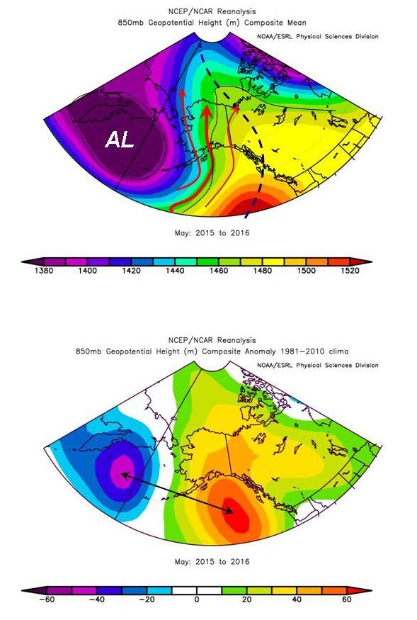
As documented by Cox et al. (2017) and highlighted in: Barrow's Annual Snow Cycle; Ecological Responses to a Lengthening Snow-free Season, snowmelt at BRW in 2015 and 2016 were the third and earliest, respectively, in the 114-year record. It is paramount to understand underlying mechanisms that result in such anomalies or to determine if these represent another shift climatologically. Through an evaluation of time series of the E-W index it was found that the advection of southerly air in May is an important factor in accelerating snowmelt. The persistence of an E-W dipole favors the flow of warm air across Alaska into the Arctic as was illustrated in Figure 6. Referring again to Figure 4, record high temperatures were observed at BRW during May of 2015 and 2016, described as heat waves (Cox et al., 2017). Figure 8 (top) shows the mean May 850 hPa field, averaged for 2015 and 2016, from the NCEP/NCAR Reanalysis. Figure 8 (bottom) is an anomaly plot that compares the 2015/2016 May field with the May 1981-2010 climatology, showing the greatly enhanced E-W pressure gradient that promotes northward advection. Flow tends to be geostrophic, i.e., following lines of constant pressure, indicated by red vectors in the top figure. The ALBSA index averaged +49 for May 2015/2016 compared with -12 for May 1986/1987, years of late snowmelt at BRW (see: Barrow's Annual Snow Cycle; Ecological Responses to a Lengthening Snow-free Season; Figure 2b). Note that average May temperatures for 1986/1987 were colder by more than 4°C than in May 2015/2016 (Figure 4).
Such patterns are not unique to spring. January 2017 was also anomalously warm in Barrow, where it "tied for the second-warmest January in the community since records there began in 1921…with an average temperature of 4.3 degrees Fahrenheit, which was 11 degrees above normal."
Contributing to the warmth was the advection of warm air from the North Pacific as is evidenced by analyzing the mean geopotential height fields for January 2017 using the NCEP/NCAR Reanalysis products. Figure 9 (top) shows the mean 850 hPa field and below is the associated vector wind field. The four ALBSA reference points, N, S, E and W, are shown in the top figure. In this case, ALBSA was > +100, a value indicative of high potential for transporting Pacific air into the Arctic as is verified by observation.
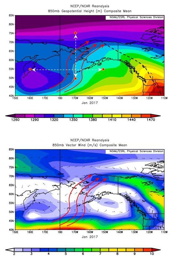
There are distinct similarities between the above examples, for May (Figure 8) and January (Figure 9). In both cases, the AL shifted to the western Bering Sea and a high pressure ridge formed over the eastern Pacific-Western Canadian region extending into Alaska. The BSA is absent. The juxtaposition of the AL and the ridge of high pressure favors the advection of warm, moist Pacific air well into the Arctic. The opposing pattern exists when the BSA is positioned north of BRW and the AL is more centrally located over the Aleutian Islands, establishing a N-S dipole as shown in Figure 5 (left). The BSA blocks the incursion of Pacific air and BRW remains cool and dry due to onshore flow of air circulating around the High. How the various patterns are manifested climatologically, their frequency, intensities and persistence, their transitions on varying time scales, have significant influence on the climate of the Pacific Arctic. Having a means to quantify the potential for the advection of Pacific air into this region of the Arctic, using an index such as ALBSA or its components, E-W and N-S, provides a valuable tool. Cox et al. (2017) applied this tool when evaluating factors that influence the snowmelt date in spring at BRW. A first step is to produce time series of these indices in order to evaluate variations and trends.
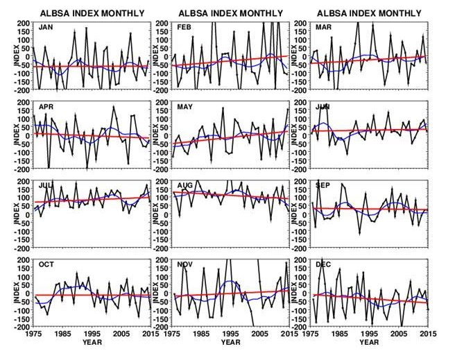
Figure 10 is a composite plot of the ALBSA index time series, by month, for the period 1975-2016, in which data have been fitted linearly and also smoothed to show trends and multi-year variations. There is considerable inter-annual variability, particularly in winter. Summer values tend to be positive while winter values are neutral or negative. When resolved by month, some show little or no change, while others show tendencies to increase or decrease in value. May is notable in that it has gone from negative to slightly positive and is known to correlate with temperatures and the timing of snowmelt at BRW. Interestingly, December shows a tendency towards more negative values while temperatures have risen quite dramatically (Figure 4). This may be due to the fact that the BSA has had a greater presence in recent years but instead of having a cooling effect, it is warming BRW due to the delay in ice formation in the Beaufort Sea resulting from greater retreat of the sea ice in summer (e.g., Cox et al., 2017).
It is suggested such analyses be cross correlated with other metrics of climate or environmental change to gain a better understanding of how synoptic-scale circulation patterns influence components of the Arctic system; be it snow, ice, phenology, permafrost, biogeochemical cycles or animal habitats. Once relationships are revealed, their time-varying linkages may be exploited to develop physically based, empirical models for the purpose of making forecasts. For instance, if there is a high correlation between the date of snowmelt at BRW and/or the onset of sea ice melt in adjacent seas with the March/April ALBSA index, sea ice conditions in summer may be better predicted than at present. NOAA personnel are investigating such prospects in collaboration with Working Groups associated with the International Arctic Systems for Observing the Atmosphere (IASOA) (https://www.esrl.noaa.gov/psd/iasoa). We note however, the indices introduced here are applicable mostly to study the Pacific Arctic region.
NOTE: Further details of the impact of synoptic-scale circulation patterns on the climate of Northern Alaska, and the response of the regional ecosystem can be found at the site:
Barrow's Annual Snow Cycle; Ecological Responses to a Lengthening Snow-free Season