1. Central Calibration Laboratory
2. CO2 Scale Report

The following is a report prepared for the 15th WMO/IAEA Meeting of Experts on Carbon Dioxide, Other Greenhouse Gases, and Related Tracer Measurement Techniques, held September 7-10, 2009 at the Max-Planck-Institute for Biogeochemistry (MPI-BGC) in Jena (Germany).

The complete transformation of our global energy infrastructure that is required to decrease the probability of potentially catastrophic global climate change is a daunting challenge. It generates much resistance while at the same time creating exciting opportunities. The need to aggressively reduce emissions (Stern, 2009) leads to a demand for reliable and objective information about emissions by country and region, by sector, and by large individual point sources. Policy makers and the public need to know to what extent policies are successful in reducing emissions. Thus our community has a new task, in addition to our traditional goals of figuring out how the biogeochemical cycles works, and how they may be affected by climate change and management practices. The new task is to quantify emissions and removals in an objective and transparent way, using combinations of improved emissions inventories and models, a dense atmospheric measurement system, atmospheric transport models and sophisticated statistical techniques. We can help create confidence in policies and transactions. The results of any observing system will surely be severely challenged because of the enormous political, financial, economic and emotional stakes involved.

General requirements of the measurements.

All measurements should be accepted as fully trustworthy, which implies complete and prompt disclosure of all results, including data flagged as faulty or not suitable for some purposes. Traditional “ownership” of data has now become obsolete, and can be (has been already) damaging to our credibility as climate scientists. Careful data management and full disclosure are not an afterthought. They are a necessity that we need to plan and provide funding for from the start. Full disclosure requires a data management system that enables full disclosure, while data management also facilitates quality control and helps maintain documentation and archival.

Since results are sensitive to relatively small differences between individual measurements, the measurements should be precise and directly comparable, as specified by the WMO (see Table 1 of the Recommendations in this report). All measurements should be traceable to the applicable WMO reference gas scale for each species. If this cannot be achieved, because of political barriers for example, other scales have to be compared to the WMO scale at regular intervals.

All reported measurements should be accompanied by defensible uncertainty estimates. A measurement without an uncertainty estimate cannot be compared to any other, even when they are all traceable to the same reference scale. Defensible uncertainty estimates require a considerable amount of duplication of measurements of actual air samples.

The WMO has recently entered into an agreement with the Bureau International des Poids et Mesures. The BIPM has as its mandate to provide the basis for a single, coherent system of measurements throughout the world, traceable to the International System of Units. Practical consequences are that our measurements acquire a certain legal standing, and that the WMO will be able to participate in regular Key Comparisons between national metrology institutes. Another desirable outcome would be that we agree to adhere to well defined and accepted terminology (VIM3, 2007; De Bièvre, 2008; Table 2 in the Recommendations). Such adherence has important practical consequences, as suggested below.

Some implications of terminology.

Measurand: Quantity intended to be measured.

Measurement result: Set of quantity values attributed to a measurand, together with any other available relevant information.

A measurement result has to include an estimate of its uncertainty, taking into account all known contributions, such as potential errors incurred in collecting the sample. A statistical estimate of repeatability, as is often reported, is incomplete and usually underestimates the uncertainty.

Measurement error: Measured quantity value minus a reference quantity value.

This definition implies that any measurement is a comparison with a measurement standard. It does not include the uncertainty associated with the reference value itself.

Measurement precision: Closeness of agreement of replicate measurements under specified conditions:

1. Repeatability: same operators, same equipment and procedure, same location, same environment, over a relatively short time period.
2. Reproducibility: different operators, equipment, procedure, location, environment, and over extended time period.

Comparability: Measurement results are comparable if they are metrologically traceable to the same reference.

Comparable does not mean that measurements results are close in magnitude, but that they are referenced to the same scale.

Traceability: Measurement results are related to a reference through a documented unbroken chain of calibrations, each contributing to the measurement uncertainty.

“Chain” is singular, not plural. When we use reference gas mixtures (such as “target” gas mixtures or “round robin” comparison mixtures) outside of our defined single hierarchical calibration chain, they provide information values, not calibrations, and can be used to verify the calibration transfer chain.

The WMO Mole Fraction Scale for CO₂.

Until this point the discussion has applied to all of the species we measure, but from here on the focus will be on CO₂ alone.

The current CO₂ scale is realized by measuring at regular intervals, about every two years, the temperature and pressure of several aliquots from each Primary high pressure cylinder filled with CO₂-in-natural-air in a well calibrated ~6 liter volume. From each air aliquot CO₂ and N₂O are then quantitatively extracted, and, after removal of trace H₂O from the extract, its pressure and temperature are measured in a small (~10 cc) calibrated volume (Zhao, 1997, 2006). After a small correction for N₂O, this procedure results in a mole fraction of CO₂, and it is called the manometric method.

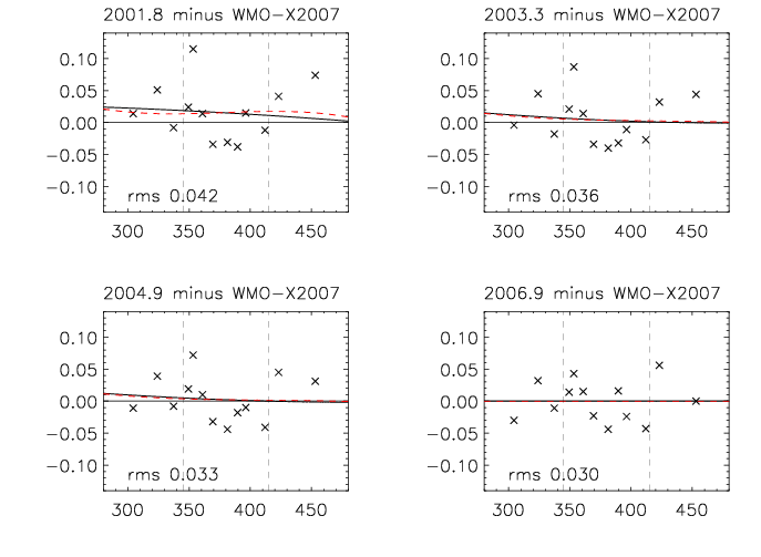
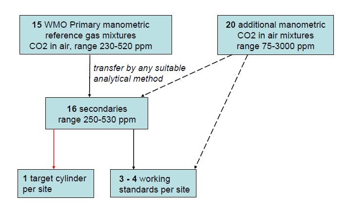
There are 15 WMO Primaries that were created by compressing dried clean ambient air at Niwot Ridge, Colorado, (altitude 3040 m) during 1990 while adjusting the CO₂ mole fraction by adding small amounts of 10% CO₂-in-air, or by trapping CO₂ during part of the filling procedure in the case of lower than ambient standards. Starting in 1991, they have been measured four times, until 1999, by C.D. Keeling at the Scripps Institution of Oceanography, which was the WMO Central Calibration Lab for CO₂ until 1995. Starting in 1996, they have until now been measured eight times on the manometric analysis system at NOAA/ESRL. Repeated measurements of the same cylinder over a long period of time offer the opportunity to check for drift over time of the CO₂ mole fraction. Thus far we have no evidence of drift, or more precisely, the null hypothesis of zero drift cannot be rejected for any of the Primaries. The assigned value of each Primary has changed a bit over time as more measurements accumulated, and thus the definition of the scale has also changed, despite us having no evidence that the mole fraction of individual Primaries has drifted. Differences of the scale after earlier calibration episodes from the X2007 scale are plotted in Figure 1. We expect to issue soon the X2010 version of the WMO Scale after we have incorporated the results of the most recent (2009) calibration episode.

Figure 1. Changes of the WMO Scale since 2001. After each calibration episode, when the value assigned to each Primary has been revised, the 13 central Primaries are all compared multiple times in quick succession on a non-dispersive analyzer, creating a relation between voltage and mole fraction. The relation, expressed as a quadratic or cubic polynomial curve fit, defines the WMO Scale on that analyzer at the time. Strictly for the purpose of calibration transfer, we then let the 13 Primaries “represent the curve” by subtracting the residuals from their individual assigned values. In the lower right the residuals of the individual assigned values relative to the curve fit are plotted after the calibration episode centered on decimal date 2006.9 which defines the X2007 version. In that case the sum of the residuals equals zero. The other three plots show differences of the assigned values of individual Primaries after earlier calibration episodes from the X2007 curve fit. Quadratic (black) or cubic (red dashed) curve fits through these earlier differences show how the WMO Scale has changed since 2001.

The WMO Scale was most recently (in 2006) compared to independent gravimetric standards made by the National Institute of Environmental Sciences, Tsukuba, Japan (Tohjima, personal communication). The average difference (gravimetric minus manometric) of five cylinders was -0.01 ppm, and standard deviation 0.02 ppm. Earlier comparisons were carried out with Scripps. Differences in the ambient range (350-420 ppm) are typically less than 0.1 ppm, but there is no finalized comparison because of some unresolved issues with the Scripps manometric system.

Transfer of the WMO Mole Fraction Scale for CO₂.

Since we want to keep the Primaries for many decades, they are used sparingly. Twice per year the WMO Scale is transferred to secondary standards, using comparative measurements on a non-dispersive infrared analyzer (Figure 2). The secondaries are used daily to calibrate all other cylinders, and they are typically used up in a few years.

Figure 2. Calibration hierarchy of the WMO Mole Fraction Scale for CO₂.

Calibrations for other labs, as well as calibrations of field standards for ESRL, are performed in almost all cases with the secondaries. At ESRL we are currently using a target cylinder, measured once every 25 hours, at field sites as a check on the calibration transfer and on potential drift of field standards. The calibration procedures at field sites have to depend on the characteristics of the analyzers that are used.

Figure 3 illustrates that the propagation of the calibration scale can be done in a precise and consistent manner. The left panel gives an idea of the precision (intermediate between conditions of repeatability and reproducibility) of transfer calibrations from the WMO Scale to field standards. Already included implicitly is a minor error component of potential drift during a few months use of a cylinder. 95% of the differences are less than 0.05 ppm, and the standard deviation is 0.024 ppm. Each difference has an equal contribution to its error from the first and the last calibration, so that the statistical uncertainty of a single transfer calibration is 0.024/√2=0.017 ppm, or 0.034 ppm at 2 sigma. The average difference of succeeding calibrations from the first is 0.008 ppm, suggesting a slight bias perhaps caused by handling. The value assigned to a cylinder is always an average of the initial calibrations. The right hand panel suggests that during up to ten years of use the probability of significant drift is small. The long-term comparisons include potential drift of individual cylinders as well as potential long-term systematic variations in the WMO scale itself and in calibration transfer procedures.

Figure 3. Left panel: Second and third calibration minus the first. Right panel: Differences of calibrations performed between one and ten years after the initial calibration(s). The number of comparisons of final calibrations performed between January 2000 and November 2009 is indicated above each bar. Statistics are based on Luxfer AL150 cylinders with CO₂ mole fractions between 350 and 450 ppm, and with final pressure above 20 bar.

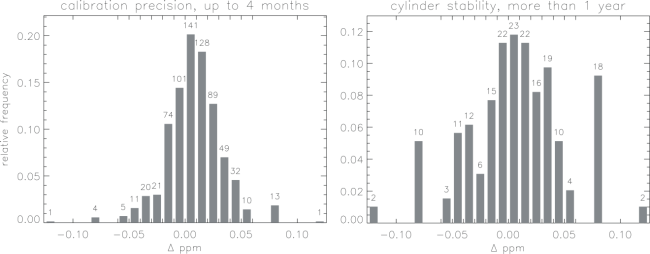
The mean difference between later calibrations and the initial one(s) is 0.007 ppm while one standard deviation of the differences is 0.043 ppm. The mean time between final and initial calibrations is 3.0 years. There is no discernable trend of the mean difference as a function of time. 80% of the cylinders differed by less than 0.05 ppm. In all cases included in Figure 3 the final cylinder pressure was still above the recommended minimum use pressure of 20 bar. However, in cases in which the final pressure was below 20 bar, the mean absolute difference increased to 0.085 ppm. We have found thorough drying of the cylinder air to be a key ingredient for stability. Small leaks can also contribute to cylinder drift.

In Figure 2 we state that the calibration transfer can be performed with “any suitable analytical method”. Ideally the transfer should not depend on which method is used. In fact, that is the basis of the method of using air mixtures to transfer the WMO Scales. Different instruments may have varying sensitivity to isotopologues of CO₂. Manometric standards include all isotopologues equally, and gas chromatography does not typically separate isotopologues, but non-dispersive infrared analyzers have different sensitivity to isotopologues, and high resolution spectral methods are often designed to be sensitive to just one. The abundance of ¹²C¹⁶O₂ as a fraction of total CO₂ is 0.9840, assuming PDB isotopic ratios for carbon and oxygen and statistical independence of multiple isotopic substitutions. In the extreme case that the scale is transferred by an instrument that is sensitive to only ¹²C¹⁶O₂, no error is made when that same instrument is used to measure outside air that happens to have the same isotopic composition as the WMO Primary standards. The assessment of errors becomes complicated if different instruments are used at different stages of the traceability chain. The errors are typically very small in most cases, as estimated below. Eq. 1 is a very good approximation of the errors, with X the mole fraction of total CO₂, ΔX the error in the measured atmospheric mole fraction,

R_air the fractional abundance in CO₂ of one isotope relative to the sum of all in the air being measured (in the case of carbon it is ¹³C/[¹²C+¹³C], for oxygen-18 it is ¹⁸O/[¹⁶O+¹⁷O+¹⁸O]), etc., and δ is defined (and expressed in permil) as the deviation of R_ref of the reference standard from R_air, specifically as (R_ref/R_air – 1) • 1000. Δδ is the mistake we make (δ_ref – δ_atm) when we assume that the isotopic composition of our reference gas is the same as in the atmosphere, or more generally, in the gas we are trying to measure which would also include a calibration transfer in a calibration chain. When Δδ is positive and the instrument is measuring ¹²C¹⁶O₂ only, there is relatively less ¹²C¹⁶O₂ in the reference gas than in the atmosphere. Then atmospheric total CO₂, the sum of all isotopologues, will be overestimated with an instrument that is only sensitive to ¹²C¹⁶O₂. For example, if CO₂ is 400 ppm the error is 0.0044 ppm per permil error in the ¹³C/¹²C isotopic ratio of the reference gas (δ_ref – δ_atm). It would take a 20 permil error to get a 0.089 error in the CO₂ measurement or in a transfer calibration. This can happen with reference gases in which the CO₂ component has been derived from burning oil or natural gas, in which case the oxygen isotopes would also be different from atmospheric CO₂. For natural gas the isotopic difference could be more than 20 permil. As mentioned above, these errors may be partially compensated depending on the calibration chain. The situation is actually more complicated for non-dispersive infrared analyzers because their sensitivity to isotopologues is often not well characterized and may vary between individual instruments (Lee, 2006; Tohjima, 2009). Our solution is to start providing isotopic ratio values for standard reference gas mixtures and for the WMO Primaries so that the isotopic composition of CO₂ is fully characterized, giving users the tools to deal with the issue in their particular situation. It is also a good idea (for us and others) to use analyzers for calibration transfer that are sensitive to the main isotopologue only, which would avoid ambiguities arising from variable and partially known instrument sensitivities to different isotopologues.

Measurement uncertainties in addition to the transfer of the calibration scale.

It should be expected, and experience shows, that the uncertainty associated with the calibration transfer chain is only one component of the overall uncertainty. The dominant component often comes from errors incurred when a sample is isolated from ambient air in order to be measured in a calibrated instrument. To quantify the mole fraction in dry air, we need to control and/or measure the temperature, pressure and flow rate of the air sample, and we need to thoroughly dry it or measure its water vapor mole fraction and correct for it. Frequent calibrations may be used to partially compensate for inadequacies of sample control. Another common source of errors is small leaks in the plumbing which could affect the calibration as well as the sampling of outside air. This list is not meant to be exhaustive, but the question is how we can quantify the uncertainties that may be caused by such errors in an efficient way. We propose that the most effective way is to compare on an ongoing basis the measurement results of ambient air between different methods and between different laboratories. One example is shown in Figure 4. When one method produces systematically higher or lower results than the other(s), larger than a predetermined target reproducibility of 0.3 ppm for example, one could decide to investigate the cause of the discrepancy and take measures to remedy the problem. Since Figure 4 is rather typical for such comparisons it also suggests that we have not been able to consistently achieve the recommended 0.1 ppm target level of agreement between atmospheric measurements. Quite apart from any remedies however, even when the cause of the systematic difference cannot be determined, the comparison produces an ongoing time-dependent statistical estimate of the reproducibility of measurements of our measurand, the CO₂ mole fraction in dry air. Such an estimate is an essential part of any measurement, without which the measurement result is incomplete.

Figure 4. Weekly duplicate flask samples, collected at the Mauna Loa Observatory in two different ways, are compared to the hourly means of a continuous analyzer during the time the flask samples were taken. Continuous lines in upper panel are moving averages through each data set of the differences. Click on image to view full size graph.

References:

• De Bièvre, Paul, Essential for metrology in chemistry, but not yet achieved: truly internationally understood concepts and associated terms (2008). Metrologia 45, 335-341.
• Tohjima, Y., K. Katsumata, I. Morino, H. Mukai, T. Machida, I Akama, T. Amari, and U. Tsunogai (2009), Theoretical and experimental evaluation of the isotope effect of NDIR analyzer on atmospheric CO₂ measurement, J. Geophys. Res. 114, D13302, doi: 10.1029/2009JD011734.
• Lee, J.-Y., H.-S. Yoo, K. Marti, D.M. Moon, J.B. Lee, and J.S. Kim (2006), Effect of carbon isotopic variations on measured CO₂ abundances in reference gas mixtures, J. Geophys. Res. 111, D05302, doi: 10.1029/2005JD006551.
• Stern, Nicholas H., The Global Deal: Climate Change and the Creation of a New Era of Progress and Prosperity, PublicAffairs press, 2009.
• VIM3, 2007 International Vocabulary of Metrology – Basic and General Concepts and Associated Terms, ISO/IEC Guide 99, 2007 (Geneva, ISO).
• Zhao, C., P.P. Tans, and K.W. Thoning (1997), A high precision manometric system for absolute calibrations of CO₂ in dry air, J. Geophys. Res. 102, 5885-5894.
• Zhao, C., and P.P. Tans (2006), Estimating uncertainty of the WMO Mole Fraction Scale for carbon dioxide in air, J. Geophys. Res. 111, D08S09, doi: 10.1029/2005JD006003.