Today’s anthropogenic climate change is largely driven by increasing greenhouse gases (GHGs) in the atmosphere, modified to some extent by the distribution of aerosols and aerosol properties. To understand the influence of changing atmospheric composition on climate change and minimize its eventual magnitude, society needs the best possible information on the trends, distributions, emissions and removals of greenhouse gases. It is necessary to develop a solid scientific understanding of their natural cycles, and how human management and the changing climate influence those cycles. Our atmospheric measurements can also provide fully transparent and objective quantification of emissions, supporting national and regional emissions reduction policies and generating trust in international agreements.
The NOAA Global Monitoring Laboratory (GML) is a world leader in producing the regional to global-scale, long-term measurement records that allow quantification of the most important drivers of climate change today. Global monitoring of atmospheric greenhouse gases, in particular carbon dioxide (CO2), has been part of NOAA’s mission for over 50 years. GML provides and interprets high-accuracy measurements of the history of the global abundance and spatial distribution of a suite of long-lived greenhouse gases. The spatial distributions, together with models of the winds and mixing (derived from weather forecasts) allow us to infer time dependent patterns of emissions/removals that are consistent with our observations. Because the measurements are calibrated they stand on their own, and can be used far into the future with better models, and also to compare with satellite retrievals of column-averaged GHGs that cannot be calibrated, but still need to be used together with calibrated data.
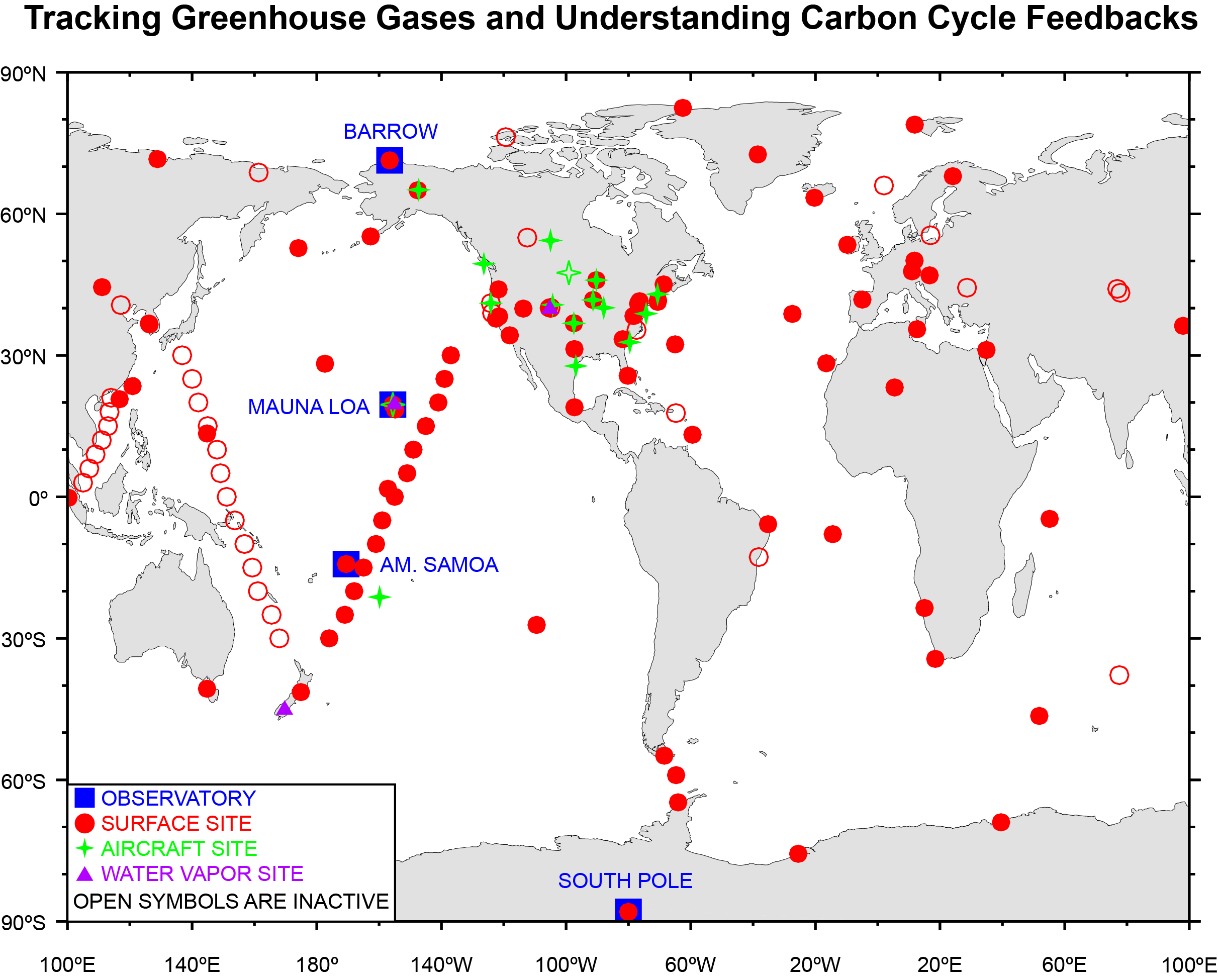
NOAA measurements of climatically important gases began in the late 1960s and expanded in the mid-to-late 1970s for CO2, nitrous oxide (N2O), chlorofluorocarbons (CFCs), and upper atmospheric water vapor. Over the years other gases and isotopic ratios have been added, including methane (CH4), carbon monoxide (CO), hydrogen (H2), numerous hydrochlorofluorocarbons (HCFCs) and hydrofluorocarbons (HFCs), methyl halides, and sulfur hexafluoride (SF6). GML produces and maintains global standards for most of the climate relevant gases. The use of common standards enables measurements by different methods, and by different countries and organizations to be used together, greatly increasing the value of the international cooperative measurement system.
Relevance: The two-way interaction between carbon sources and sinks and climate is a first-order uncertainty in predicting climate in the 21st century and beyond. Understanding the past trajectories and current state of GHG sources and sinks is a prerequisite for predicting those in the future.
Actions Taken: GML has used its long-term atmospheric observations of GHGs to quantify present day sources and sinks for three decades. Among other methods, we employ the CarbonTracker data assimilation systems for CO2 and CH4 to calculate global, continental, and regional sources and sinks. In order to improve the accuracy of our continental and regional source and sink calculations, we have increased the density of measurements over the U.S. and improved the resolution and quality of the atmospheric models we use to interpret the data.
What we’ve discovered: Global CO2 sinks have stayed roughly constant as a fraction of emissions over the past 50 years. U.S. sinks absorb about one third of U.S. fossil fuel emissions, though with large variability. Global CH4 emissions have increased since 2007 after having been steady for the preceding decade. Our measurements of CH4 isotopes imply that increased leaks from oil and gas operations are very likely not the main cause. Thus far, we have seen no evidence for dramatic increases in CH4 emissions from Arctic warming.
Relevance: These GHG emissions are responsible for anthropogenic climate change, yet the world currently relies only on self-reported, accounting-based approaches to determine emissions. Further, understanding carbon cycle response to climate change requires separation of human and ecosystem influence. We are developing techniques that allow objective and transparent quantification of emissions using atmospheric data.
Actions Taken: In addition to the long-term measurements of GHGs mentioned above, GML has measured the atmospheric content of species like 14CO2, CO, and other gases directly related to anthropogenic emissions, especially in the North American part of our network. These measurements have been used to estimate emissions of a variety of different trace gases. For example, in the case of anthropogenic methane emissions in the U.S., we have conducted short duration (weeks) intensive campaigns in and around oil and gas extraction regions. Longer duration (years) studies have also been performed around cities in order to estimate fossil fuel-CO2 emissions. We have done Observation System Simulation Experiments (OSSEs) to help design the observational and modeling frameworks needed to most effectively use atmospheric data to estimate emissions.
What we’ve discovered: Atmospheric measurements of the strong GHG SF6 have shown that inventories (from “bottom-up” accounting) greatly underestimate global emissions. Increases of CH4 emissions over the U.S. have been, at most, modest during the last decade. Based on our δ13C data, global emissions of CH4 from fossil fuel use are a larger fraction of total anthropogenic emissions than previously believed, while the recent increase of atmospheric CH4 is likely not due to increased fossil fuel emissions. Our estimate for U.S. HFC-134a emissions is consistent with the EPA inventory, while our observations for CCl4 indicate that U.S. emissions are more than a factor of ten larger than the EPA’s Toxics Release Inventory.
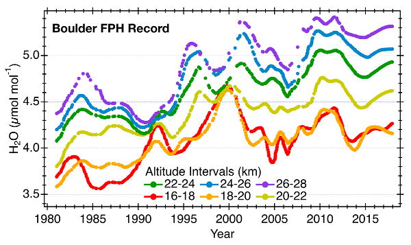
Relevance: Changes in water vapor abundance near the tropopause exert a strong influence on climate. For example, if the 25% increase in stratospheric water vapor observed over Boulder between 1980 and 2010 is representative of a global trend, it would be responsible for enhancing the rate of surface warming by 30% during the 1990s.
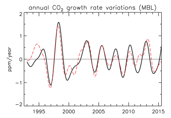
Actions Taken: Monthly water vapor soundings with balloon-borne frost point hygrometers (FPHs) were initiated in 1980 at Boulder and in 2004 at Lauder, New Zealand. Realizing a compelling need for water vapor vertical profiles in the tropics, monthly FPH soundings began in 2010 at Hilo, Hawaii. Time series of stratospheric water vapor mixing ratios produced from these soundings were analyzed for long-term trends and compared to measurements by satellite-based water vapor sensors. The Hilo data also help us better understand interannual changes in the tropical tropopause layer (TTL) that are driven by dynamical processes like the Quasi-Biennial Oscillation (QBO), the El Niño-Southern Oscillation (ENSO) and the Brewer-Dobson circulation (BDC). Smoothed, detrended annual mean growth rate of CO2 derived from the Marine Boundary Layer (MBL) subset of sites (black line) and the same CO2 growth rate derived from the observed 13C/12C ratios of CO2 at the MBL sites, assuming that the isotopic signature is characteristic of photosynthesis by land plants (dashed red line). The fairly close match between the lines demonstrates that the CO2 growth rate variations are almost entirely due to terrestrial ecosystems, not to the oceans.
What we’ve discovered: Stratospheric water vapor over Boulder has increased by approximately 25% since 1980. Only one-third of this long-term trend can be attributed to increasing amounts of methane entering the tropical stratosphere where it is oxidized to water vapor suggesting this may be a strong climate feedback. Satellite-based measurements of stratospheric water vapor provide better spatial coverage of the globe than FPH soundings but are often fraught with biases and temporal drifts, and, so far have been unable to provide reliable, long-term trends. The value of the near-global satellite records can be greatly enhanced once their biases and drifts have been characterized using FPH profiles.