Instructions for Monthly/Seasonal Climate Composites
Page will plot maps or vertical crosdivs of selected variables. Select desired options and hit "create plot". Most options have a default setting so a selection is not required. Default for year is last year and month available for dataset. you can select one or more years to composite, the season, the type of statistic plotted (mean, anomaly, climatology), variable, level, map color, map location or bounds for vertical composites and contour interval/range. If you have problems, please email with ALL the options you chose.
Please read ALL the instructions. Failure to do so may lead to misinterpretation of results.
Variable, Years and Levels Available TopGo to Page Top
Data is available from Jan 1948 to the present for most variables and is updated the first or 2nd week of the month with the previous month's data.
ONLY pressure and air temperature are available for the tropopause level and ONLY u and v winds, relative humidity and pressure for the surface. Streamfunction, divergence, vorticity and velocity potential are available ONLY on sigma levels.
Vector Winds: Magnitude of winds are contoured. Arrows show direction.
Sea Surface Temperature: This is from the NOAA OI SST data (prescribed). Over land it is the skin temperature (prescribed as well). Sea Ice (which varies near land) affects these values and so the plotting range may not be as great over the tropics as desired. Using a lower latitude may help with the plot.
Enter Years TopGo to Page Top
Enter each year in a separate box. The year should correspond to the last month of a season. Years should be within the range of the dataset you select. You can subtract one set of years from another by entering a negative year.
Enter Range of Years TopGo to Page Top
Enter a range of years within the range of the data. You can also enter a range of years or use a time series or list of years (see next entry).
List of Years TopGo to Page Top
You can use a file containing the years you would like. The format is:
        # of years
        year1
        year2
        year3
        ...
        lastyear
Ftp to ftp2.psl.noaa.gov as anonymous. Please deposit your time series in /Public/incoming/timeseries using a unique name. Type in full pathname (/Public/incoming/timeseries/yourfilename where requested.
Compositing Off a Time Series TopGo to Page Top
You may select a time series or enter one yourself. Details on the supplied ones are at Climate Index Web Page for a complete reference for the included time series. Credit, proper references and definitions are provided. Please read before using a particular time series or you may misinterpret what you are seeing. You can use the web page http://psl.noaa.gov/data/timeseries/ to create your own from monthly mean datasets. For ENSO years, see the PSL's ENSO FAQ.
To use you own or one obtained from the /Timeseries/ web page, ftp to ftp2.psl.noaa.gov as anonymous. Place time series in /Public/timeseries using a unique name. Check the "list of years" box and those years will be used. To use a time series, ftp a file to the same directory as above. However, the format is:
        yearstart yearend
        year1 val1 val2 val3 val4 val5 val6 val7 val8 val9 val10 val11 val12
        year2 val1 val2 val3 val4 val5 val6 val7 val8 val9 val10 val11 val12
        etc
        yearend  val1 val2 val3 val4 val5 val6 val7 val8 val9 val10 val11 val12
        missing value
The missing value is mandatory and cannot be in the range of the data (-9999 is a good one). Select "custom" time series.
For either a supplied time series or your own, you can composite off the actual values, anomalies (mean is based on the complete range of years of the time series you submit or use, standardized anomalies (anomalies divided by the standard deviation), or the percentile (0 to 100). Years used for composites are the subset of those years which match the criteria AND are in the dataset you choose. For example, if you choose a Nino3.4 time series that has values greater than 1.5 sigma and the dataset you are looking at goes to 1995, you will NOT get 1998 even if the Nino3.4 value is greater than 1.5 sigma.
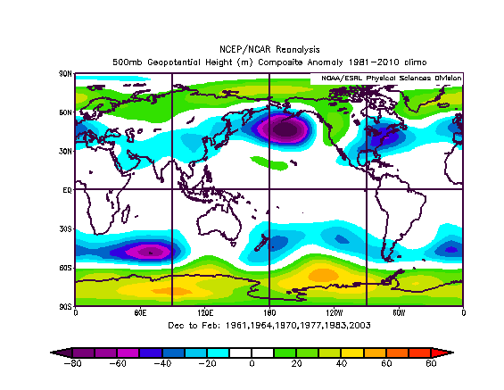
For a concrete example, let's composite 500mb geopotential height for winter seasons (Dec-Jan-Feb) where the PNA index exceeds 1.25 sigma.
- Choose geopotential height
- Choose 500mb level
- Select "Years from values in Time Series"
- Select timeseries "PNA"
- Select "standardized anomaly"
- Select "greater than or equal to"
- Select "anomaly"
- Select "all" for map
- Select "create plot"
- Choose default (make no selection) for other options
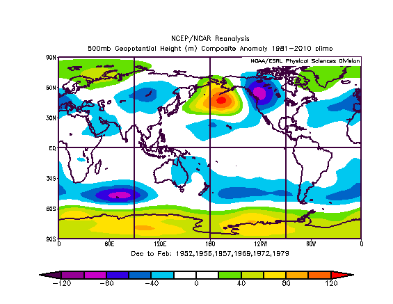
Note: There are 6 years returned (using 1948-Nov 2013 data): 1961, 1964, 1970, 1977, 1983, 2003 The typical 3 center pattern over North America clear is visible. Now, try years less than or equal to -1.25 sigma. Only 5 years are returned: 1952,1956,1957,1969, 1972,1979 and the plot is somewhat opposite in pattern. You results may vary as more years are added to the PNA and the NCEP data.
Lagged Composites TopGo to Page Top
Selecting a nonzero value for this will allow you to do a lagged composite. The years are determined from one of the year entry methods above. Then, a composite is made N months before the dates you selected (-N) or after the dates you selected (N). If lagging results in a date that is not in the range of the dataset, that date is not used. As an example, select January 500 geopotential height for the PNA values greater than 1.25 sigma. If you choose lag =-1, you will get 5 years: 1977, 1981, 1985, 1992. A negative lag of one month will composite geopotential height for Dec 1976, 1980, 1984, 1991. A positive lag of 3 months will composite for April of 1976, 1980, 1984, 1991. All lags are specified in months!. Please do lags only on positive years.
How the Composite is Calculated TopGo to Page Top
The composite represents the average of the variable for all months and years entered. Composites can be created for one set of years minus another. The years are normalized as in the following example: a set of 5 years minus a set of 2...
(1980+1981+1982+1983+1984)-(1985+1986)
will be calculated as...
(1980+1981+1982+1983+1984)/5.-(1985+1986)/2
...where each year represents a monthly/seasonal value. There is currently no data before 1948 for reanalysis so, for example, the season DJF 1948 contains Dec 1947 and therefore will not be calculated. Likewise, seasons that would have years after the end of a dataset will not be calculated. Missing values will not be used for data outside the time range of the dataset.
Rotating Plots TopGo to Page Top
To rotate map, choose "custom" map projection and then choose either northern or southern polar stereographic projection. For lat range, enter 0 to 90 (for northern hemisphere) or -90 to 0 for southern. For longitude, the center of the longitude range input will be at the bottom of the plot. To center along 0E, choose -180 to 180, for example. To center at 90E, choose -90 to 270. You can plot sectors as well. The longitudes -90 to 90 in the NH will plot the half hemisphere from the US across the Atlantic to Europe.
Type of Plot TopGo to Page Top
- Mean
- Plots are averages of all months and years that are input.
- Climatology
- Plots are based on 1981-2010 climatologies for NCEP Reanalysis data. Some other datasets have different climatology time periods. Choose season; years are not needed. If years are entered, they are ignored.
- Anomaly
- Plots are of mean-climatology for each season/month. Climatology time period is generally on 1981-2010 though some datasets have a different climatology period. For SST data from the reanalysis, anomalies can be large in the mid to upper latitudes as sea ice influences the data. Hence, you may need to restrict the range that is plotted.
Reverse Color Bar TopGo to Page Top
By typing in negative years (e.g. -1983 and not 1983), the color bar will be reversed since you will be getting -1 times the value (either mean or anomaly).
Contour Options TopGo to Page Top
A desired contour interval and range can be input instead of the default being used. Different plots can be easily compared (and the resulting gifs could be animated). For this option to work, the interval AND the range must be input. There must be at least 2 and less than 33 contours. The contour interval must be positive and the range must go from low to high.
Black and White Option: Black and white contours and shading are available for use on non-color printers.
Plotting Regions TopGo to Page Top
- Maps
- To plot over the dateline, use values from 0 to 720. For example, to plot 180W eastward to 180W, use 180 to 540. Be sure that the western most longitude is less than the eastern., For example, to plot 100W to 70W, use -100 to -70 or 260 to 290 and NOT 100 to 70.
There are 6 custom projections:
- Northern Hemisphere: 0-90N, 0-360W in using a polar stereographic projection.
- Globe: 90S-90N 0E-360W
- United States: 20N-65N; 235-285 polar stereographic projection
- Tropics: 35S-35N (changed from 60S-60N)
- Tropical Pacific: 35N-35S 100E to 60W
- 4-corner States of the Western US:31-42.5N, 244.5-258.5W CO,UT,AZ,NM
- Indio-Pacific (20S-20N,60E-160W)
Height by Latitude or Longitude Cross Divs TopGo to Page Top
You can also plot cross divs of data Latitude by Height: Choose latitude/height or longitude /height for map type. Chose longitudes to be averaged over and latitude range to be displayed. Also choose level range. Only variables available at different levels can be plotted this way: (geopotential height, air temperature, relative humidity, specific humidity, potential temperature, winds and omega.
Longitude by Height: Chose latitudes to be averaged over and longitude range to be shown. Note that humidity variables only go through 300mb and omega only goes to 100mb.
How this Page was Created TopGo to Page Top
The main interface for this page is an html form. The data that are input into this form are processed by a Perl script. The script reads the inputs, tests for bad inputs and then executes a FORTRAN code that produces a composite file (in netCDF). This file is what is processed by a GrADS script. The GrADS script is run as a batch job. Plot options are input into the GrADS script. The plot in the frame buffer is converted to gif and this gif is displayed as part of a html document. The netCDF file and the gif file are kept in a directory where the files are periodically deleted.