3.1. Aerosol Monitoring

D. Delene (Editor), E. Andrews, D. Jackson, A. Jefferson, J. Ogren, P. Sheridan, and J. Wendell

3.1.1. Scientific Background

Aerosol particles affect the radiative balance of Earth both directly, by scattering and absorbing solar and terrestrial radiation, and indirectly, through their action as cloud condensation nuclei (CCN) with subsequent effects on the microphysical and optical properties of clouds. Evaluation of the climate forcing by aerosols, defined here as the perturbation of the Earth's radiation budget induced by the presence of airborne particles, requires knowledge of the spatial distribution of the particles, their optical and cloud-nucleating properties, and suitable models of radiative transfer and cloud physics. Obtaining a predictive relationship between the aerosol forcing and the physical and chemical sources of the particles additionally requires knowledge of regional and global-scale chemical processes, physical transformation, and transport models for calculating the spatial distributions of the major chemical species that control the optical and cloud-nucleating properties of the particles. Developing and validating these various models requires a diverse suite of in situ and remote observations of the aerosol particles on a wide range of spatial and temporal scales.

Aerosol measurements began at the CMDL baseline observatories in the mid-1970s as part of the Geophysical Monitoring for Climatic Change (GMCC) program. The objective of these "baseline" measurements was to detect a response, or lack of response, of atmospheric aerosols to changing conditions on a global scale. Since the inception of the program, scientific understanding of the behavior of atmospheric aerosols has improved considerably. One lesson learned is that residence times of tropospheric aerosols are generally less than 1 week, and that human activities primarily influence aerosols on regional/continental scales rather than global scales. In response to this increased understanding, and to more recent findings that anthropogenic aerosols create a significant perturbation in the Earth's radiative balance on regional scales [Charlson et al., 1992; National Research Council, 1996], CMDL expanded its aerosol research program to include regional aerosol monitoring stations. The goals of this regional-scale monitoring program are: (1) to characterize means, variabilities, and trends of climate-forcing properties of different types of aerosols, and (2) to understand the factors that control these properties.

A primary hypothesis to be tested by NOAA's aerosol research program is that the climate forcing by anthropogenic sulfate will change in response to future changes in sulfur emissions. The forcing is expected to decrease in and downwind of the United States as a result of emission controls mandated by the Clean Air Act, while continued economic development in China and other developing countries is expected to lead to an increased forcing in and downwind of those areas. Testing this hypothesis will require a coordinated research program involving modeling, monitoring, process, and closure studies. This report describes the observations that CMDL is conducting towards this goal.

No single approach to observing the atmospheric aerosol can provide the necessary data for monitoring all the relevant dimensions and spatial/temporal scales necessary to evaluate climate forcing by anthropogenic aerosols. In situ observations from fixed surface sites, ships, balloons, and aircraft can provide very detailed characterizations of the atmospheric aerosol but on limited spatial scales. Remote sensing methods from satellites, aircraft, or from the surface can determine a limited set of aerosol properties from local to global spatial scales, but they cannot provide the chemical information needed for linkage with global chemical models. Fixed ground stations are suitable for continuous observations over extended time periods but lack vertical resolution. Aircraft and balloons can provide the vertical dimension, but not continuously. Only when systematically combined can these various types of observations produce a data set where point measurements can be extrapolated with models to large geographical scales where satellite measurements can be compared to the results of large-scale models, and where process studies have a context for drawing general conclusions from experiments conducted under specific conditions.

Measurements of atmospheric aerosols are used in three fundamentally different ways for aerosol/climate research: algorithm development for models and remote-sensing retrievals, parameter characterization, and model validation. Laboratory and field process studies guide the development of parameterization schemes and the choice of parameter values for chemical transport models that describe the relationship between emissions and concentration fields of aerosol species. Systematic surveys and monitoring programs provide characteristic values of aerosol properties that are used in radiative transfer models for calculating the radiative effects of the aerosols, and for retrieving aerosol properties from satellites and other remote sensing platforms. And finally, monitoring programs provide spatial and temporal distributions of aerosol properties that are compared to model results to validate the models. Each of these three modes of interaction between applications and measurements require different types of data and entail different measurement strategies. Ogren [1995] applied the thermodynamic concept of “intensive” and “extensive” properties of a system to emphasize the relationship between measurement approach and applications of aerosol observations.

Intensive properties do not depend on the amount of aerosol present and are used as parameters in chemical transport and radiative transfer models (e.g., atmospheric residence time, single-scattering albedo). Extensive properties vary strongly in response to mixing and removal processes and are most commonly used for model validation (e.g., mass concentration, optical depth). Intensive properties are more difficult and expensive to measure than extensive properties because they generally are defined as the ratio of two extensive properties. As a result, different measurement strategies are needed for meeting the data needs of the various applications. Measurements of a few carefully chosen extensive properties, of which aerosol optical depth and species mass concentrations are prime candidates, are needed in many locations to test the ability of the models to predict spatial and temporal variations on regional to global scales and to detect changes in aerosol concentrations resulting from changes in aerosol sources. The higher cost of determining intensive properties suggests a strategy of using a limited number of highly-instrumented sites to characterize means and variabilities of intensive properties for different regions or aerosol types, supplemented with surveys by aircraft and ships to characterize the spatial variability of these parameters. CMDL's regional aerosol monitoring program is primarily focused on characterizing intensive properties.

CMDL's measurements provide ground truth for satellite measurements and global models, as well as key aerosol parameters for global-scale models (e.g., scattering efficiency of sulfate particles and hemispheric backscattering fraction). An important aspect of this strategy is that the chemical measurements are linked to the physical measurements through simultaneous, size-selective sampling that allows the observed aerosol properties to be connected to the atmospheric cycles of specific chemical species.

3.1.2. Experimental Methods

Extensive aerosol properties monitored by CMDL include condensation nucleus (CN) concentration, aerosol optical depth (d), and components of the aerosol extinction coefficient at one or more wavelengths (total scattering s_sp, backwards hemispheric scattering s_bsp, and absorption s_ap). At the regional sites, size-resolved impactor and filter samples (submicrometer and supermicrometer size fractions) are obtained for gravimetric and chemical (ion chromatograph) analyses. All size-selective sampling, as well as the measurements of the components of the aerosol extinction coefficient at the regional stations, is performed at a low, controlled relative humidity (<40%) to eliminate confounding effects due to changes in ambient relative humidity. Data from the continuous sensors are screened to eliminate contamination from local pollution sources. At the regional stations, the screening algorithms use measured wind speed, direction, and total particle number concentration in real-time to prevent contamination of the chemical samples. Algorithms for the baseline stations use measured wind speed and direction to exclude data that are likely to have been locally contaminated.

Prior to 1995, data from the baseline stations were manually edited to remove spikes from local contamination. Since 1995 an automatic editing algorithm has been applied to the baseline data in addition to manual editing of local contamination spikes. For the baseline stations (BRW, Mauna Loa, Hawaii (MLO), American Samoa (SMO), and South Pole, Antarctica (SPO), as well as Sable Island (WSA)), data are automatically removed when the wind direction is from local sources of pollution (such as generators and buildings) as well as when the wind speed is less than a threshold value (0.5-1 m s^-1). In addition, at MLO data for upslope conditions (1800-1000 UTC) are excluded since the airmasses do not represent “background” free tropospheric air for this case. A summary of the data editing criteria is given in Table 3.1.

Integrating nephelometers are used to determine the light scattering coefficient of the aerosol. These instruments operate by illuminating a fixed sample volume from the side and observing the amount of light that is scattered by particles and gas molecules in the direction of a photomultiplier tube. The instrument integrates over scattering angles of 7-170°. Depending on the station, measurements are performed at three or four wavelengths in the visible and near-infrared. Newer instruments allow determination of the hemispheric backscattering coefficient by using a shutter to prevent illumination of the portion of the instrument that yields scattering angles less than 90°. A particle filter is inserted periodically into the sample stream to measure the light scattered by gas molecules; which is subtracted from the total scattered signal to determine the contribution from the particles alone. The instruments are calibrated by filling the sample volume with CO₂ gas which has a known scattering coefficient.

TABLE 3.1. Data Editing Summary for NOAA
Baseline and Regional Stations

Station	Editing	Clean Sector
South Pole	a,b,c	0° < WD < 110°, 330°<WD < 360°
Samoa	a,b,c	0° < WD < 165°, 285°<WD < 360°
Mauna Loa	a,b,c,d	90° < WD < 270°
Barrow	a,b,c	0° < WD < 130°
Sable Island	a,b,c	0° < WD < 35°, 85° < WD < 360°
Southern Great Plains	a
Bondville	a

a: Manual removal of local contamination spikes;

b: Automatic removal of data not in clean sector;

c: Automatic removal of data for low wind speeds;

d: Removal of data for upslope wind conditions;

WD: Wind direction.

The aerosol light absorption coefficient is determined with a continuous light absorption photometer. This instrument continuously measures the amount of light transmitted through a quartz filter, while particles are being deposited on the filter. The rate of decrease of transmissivity, divided by the sample flow rate, is directly proportional to the light absorption coefficient of the particles. Newer instruments were calibrated in terms of the difference of light extinction and scattering in a long-path extinction cell, for laboratory test aerosols. Instruments at the baseline stations (aethalometers, Magee Scientific, Berkley, California) were calibrated by the manufacturer in terms of the equivalent amount of black carbon (BC) from which the light absorption coefficient is calculated assuming a mass absorption efficiency of the calibration aerosols of 10 m² g^-1.

Particle number concentration is determined with a CN counter that exposes the particles to a high supersaturation of butanol vapor. This causes the particles to grow to a size where they can be optically detected and counted. The instruments in use have lower particle-size detection limits of 10-20 nm diameter.

Summaries of the extensive measurements obtained at each site are given in Tables 3.2 and 3.3. Table 3.4 lists the intensive aerosol properties that can be determined from the directly-measured extensive properties. These properties are used in chemical transport models to determine the radiative effects of the aerosol concentrations calculated by the models. Inversely, these properties are used by algorithms for interpreting satellite remote-sensing data to determine aerosol amounts based on measurements of the radiative effects of the aerosol.

TABLE 3.2. CMDL Baseline Aerosol Monitoring Stations (Status as of December 1999)

Category	Baseline Arctic	Baseline Free Troposphere	Baseline Marine	Baseline Antarctic
Location	Point Barrow	Mauna Loa	American Samoa	South Pole
Designator	BRW	MLO	SMO	SPO
Latitude	71.323ºN	19.539ºN	14.232ºS	89.997ºS
Longitude	156.609ºW	155.578ºW	170.563ºW	102.0ºE
Elevation (m)	8	3397	77	2838
Responsible Institute	CMDL	CMDL	CMDL	CMDL
Status	Operational 1976. Major upgrade 1997.	Operational 1974	Operational, 1977	Operational, 1974
Sample RH	RH <40%	Uncontrolled	Uncontrolled	Uncontrolled
Sample Size Fractions	D<1 µm D<10 µm	Uncontrolled	Uncontrolled	Uncontrolled
Optical measurements	s_sp(3l), s_bsp(3l), s_ap(1l)	s_sp(3l), s_ap(1l), d(6l)	none	s_sp(4l)
Microphysical measurements	CN concentration	CN concentration	CN concentration	CN concentration
Chemical measurements	Major ions, mass	None	None	None

TABLE 3.3. CMDL Regional Aerosol Monitoring Sites (Status as of December 1999)

Category	Perturbed Marine	Perturbed Continental	Perturbed Continental
Location	Sable Island, Nova Scotia, Canada	Bondville, Illinois	Lamont, Oklahoma
Designator	WSA	BND	SGP
Latitude	43.933ºN	40.053ºN	36.605ºN
Longitude	60.007ºW	88.372ºW	97.489ºW
Elevation (m)	5	230	315
Responsible Institute	CMDL	CMDL	CMDL
Collaborating Institute	AES Canada, NOAA/PMEL	University of Illinois, Illinois State Water Survey	DOE/ARM
Status	Operational, August 1992	Operational, July 1994	Operational, July 1996
Sample RH	RH <40%	RH <40%	RH <40%
Sample Size Fractions	D<1 µm, D<10 µm	D<1 µm, D<10 µm	D<1 µm, D<10 µm
Optical measurements	s_sp(3l), s_bsp(3l) s_ap(1l)	s_sp(3l), s_bsp(3l), s_ap(1l)	s_sp(3l),s_bsp(3l), s_ap(1l), d(7l)
Microphysical measurements	CN concentration	CN concentration	CN, n(D) concentration
Chemical measurements	Major ions, mass	Major ions, mass	None

TABLE 3.4. Intensive Aerosol Properties Derived From CMDL Network

Properties	Description
å	The Ångström exponent, defined by the power-law s_spµl^-å, describes the wavelength-dependence of scattered light. In the figures below, å is calculated from measurements at 550 and 700 nm wavelength. Situations where the scattering is dominated by submicrometer particles typically have values around 2, while values close to 0 occur when the scattering is dominated by particles larger than a few microns in diameter.
w_o	The aerosol single-scattering albedo, defined as s_sp/(s_ap + s_sp), describes the relative contributions of scattering and absorption to the total light extinction. Purely scattering aerosols (e.g., sulfuric acid) have values of 1, while very strong absorbers (e.g., elemental carbon) have values around 0.3.
g, b	Radiative transfer models commonly require one of two integral properties of the angular distribution of scattered light (phase function): the asymmetry factor g or the hemispheric backscatter fraction b. The asymmetry factor is the cosine-weighted average of the phase function, ranging from a value of -1 for entirely backscattered light to +1 for entirely forward-scattered light. The hemispheric backscatter fraction b is defined as s_bsp/s_sp.
a_i	The mass scattering efficiency for species i, defined as the slope of the linear regression line relating s_sp and themass concentration of the chemical species, is used in chemical transport models to evaluate the radiative effects of each chemical species prognosed by the model. This parameter has typical units of m² g^-1.

3.1.3. Annual Cycles

The annual cycles of aerosol optical properties for the four baseline and three regional stations are illustrated in Figure 3.1 and Figure 3.2. The data are presented in the form of box and whisker plots that summarize the distribution of values. Each box ranges from the lower to upper quartiles with a central bar at the median value, while the whiskers extend to the 5th and 95th percentiles. The statistics are based on hourly averages of each parameter for each month of the year, also shown are the annual statistics for the entire period of record. A horizontal line is given that intersects the annual median so measurements above and below the median can be easily discerned.

In general, changes in long-range transport patterns dominate the annual cycles of the baseline stations. For BRW, the highest values of CN, ssp, and sap are observed during the spring arctic haze period when anti-cyclonic activity transports pollution from the lower latitudes of Central Europe and Russia. A more stable polar front characterizes the summertime meteorology. High cloud coverage and precipitation scavenging of accumulation mode (0.1-1.0 mm diameter) aerosols account for the annual minima in ssp and sap from June to September. In contrast, CN values have a secondary maximum in the late summer which is thought to be the result of sulfate aerosol production from gas to particle conversion of DMS oxidation products from local oceanic emissions [Radke et al., 1990]. The aerosol single-scattering albedo displays little annual variability, which is indicative of highly scattering sulfate and seasalt aerosol. A September minimum is observed in å when ssp and accumulation mode aerosols are also low but when primary production of coarse mode seasalt aerosols from open water is high.

For MLO, the highest ssp and sap values occur in the springtime and result from the long-range transport of pollution and mineral dust from Asia. However, little seasonality is seen in CN concentrations at MLO, indicating that the smallest particles (<0.1 mm diameter), which usually dominate CN concentration, are not enriched during these long-range transport events. Both the aerosol ssp and Ångström exponent display seasonal cycles at SPO with a ssp maximum and an å minimum in winter associated with the transport of coarse mode seasalt from the Antarctic coast to the interior of the continent. The summertime peaks in CN and å are associated with fine mode sulfate aerosol and correlate with a seasonal sulfate peak found in the ice core presumably from coastal biogenic sources [Bergin et al., 1998]. The aerosol extensive properties at SMO display no distinct seasonal variation. Albedo values above one that are evident at BRW and MLO are due to instrument noise at low aerosol concentration. These high albedo values are not present in daily averaged data. Furthermore, these high albedo value go away if you exclude data where s_sp is below 1 Mm^-1. Hence, the high albedo values result from a instrument detection limitation problem.

Based on only 4-7 years of measurements, the annual cycles for the regional stations are less certain than those of the baseline stations. The proximity of the regional sites to North American pollution sources is apparent in the results, with a monthly median values of s_sp that is nearly two orders of magnitude higher than values from the baseline stations. The Bondville site (BND), situated in a rural agricultural region, displays autumn highs in s_ap and a low in w_o which coincide with anthropogenic and dust aerosols emitted during the harvest. As evident in the lower s_sp and s_ap values, the Southern Great Plains site (SGP) is more remote than BND. SGP has a similar but less pronounced annual cycle with late summer highs in s_sp and s_ap, and a corresponding minimum in w_o. Little seasonal variability is observed in aerosol properties at WSA. Values of å tend to be higher in the summer and likely result from transport of fine mode sulfate aerosol from the continent and lower coarse-mode production of particles with lower summer wind speeds.

3.1.4. Long-term Trends

Long-term trends in CN concentration, s_sp, s_ap, w₀, and å are plotted in Figure 3.3 for the baseline observatories. The monthly means are plotted along with a linear trend line fitted to the data. The aerosol properties at BRW exhibit an annual decrease in s_sp of about 2% per year since 1980. This reduction in aerosol scattering has been attributed to decreased anthropogenic emissions from Europe and Russia [Bodhaine, 1989] and is most apparent during March when the Arctic haze effect is largest. The corresponding decrease in the Ångström exponent over the same time period points to a shift in the aerosol size distribution to a larger fraction of coarse mode seasalt aerosol. Stone [1997] noted a long-term increase in surface temperatures and cloud coverage at BRW from 1965-1995 which derive from changing circulation patterns and may account for the reduction in s_sp by enhanced scavenging of accumulation mode aerosols.

In contrast to the reduction in s_sp at BRW, CN con-centrations, which are most sensitive to particles with diameters <0.1 mm, have increased since 1976. There seems to be an offset in CN concentration starting in 1998 which corresponds to a change to a new CN sampling inlet. A step increase in late 1991 dominates the trend in CN concentration at MLO. The step increase in CN at SPO in 1989 is due to replacement of the CN counter with a butanol-based instrument with a lower size detection limit. The reason for the decrease in CN and increase in å at SMO is not readily apparent, but it could stem from changes in long-term circulation patterns.

Previous reports describing the aerosol data sets include: BRW: Bodhaine [1989, 1995]; Quakenbush and Bodhaine [1986]; Bodhaine and Dutton [1993]; Barrie [1996]; MLO: Bodhaine [1995]; SMO: Bodhaine and
DeLuisi [1985]; SPO: Bodhaine et al. [1986, 1987, 1992]; Bergin et al. [1998]; WSA: McInnes et al. [1998].

3.1.5. Special Studies

Comparison of Aerosol Light Scattering and Absorption Measurements at Barrow, Alaska From October, 1997 to October, 1999

NOAA’s Climate Monitoring and Diagnostics Lab (CMDL) has measured both aerosol light scattering (since 1976) and aerosol light absorption (since 1988) at Barrow, Alaska (BRW). To obtain data representative of clean baseline conditions, measurements from the polluted sector, defined by wind speed and direction, are automatically removed from the data set. Table 3.5 lists the instruments and their period of operation at Barrow. Initially, light scattering was measured using a 4 wavelength nephelometer and light absorption was measured using an aethalometer. This original sampling system did not include size or relative humidity control of the aerosol sample. In the fall of 1997 new light scattering and absorption instruments were installed at Barrow (within 2 meters of the old instruments). The new instruments are designated NSA (for North Slope, Alaska) to distinguish them from the co-located BRW instruments. The new system obtains measurements at two size cuts by using a valve to switch between a 10 mm and 1 mm impactor. Relative humidity is maintained at or below 40% by heating the air sample. The BRW and NSA systems were operated simultaneously for approximately 1 year (Fall, 1997 – Fall, 1998). One year of simultaneous light scattering measurements and two years of light absorption measurements from the co-located instruments are compared. It is important to understand how measurements from these instruments compare in order to maintain data consistency for the entire measurement period.

The comparison procedure was:

· Select data for the overlap period October, 1997 to October, 1998 for s_sp; October, 1997 to October, 1999 for s_ap.

· Estimate the absorption coefficient for the aethalometer using: s_ap = 10 m²/g * [BC]

· Apply quality control edit corrections to data sets (e.g., remove spikes and contaminated data)

· For the NSA data set, use only 10 mm size cut data.

· Correct the NSA PSAP data for: (a) scattering by particles within the filter and (b) spot size. Also, remove low transmittance data (e.g. transmittance < 0.5 as per [Bond et al.,1999]

· Calculate hourly averages of scattering and absorption coefficients

· Calculate daily averages of absorption for the aethalometer and PSAP

· Remove obvious outliers (four points for the s_ap data).

· Determine the least squares linear fit and correlation coefficient for the data sets. Perform the regression for both a calculated and forced-to-zero y-intercept.

Figure 3.4 shows that, for the two years, on an hourly basis, there is a relatively low correlation between the PSAP and aethalometer measurements (R²=0.70) although the instruments agree fairly well – the slope is 0.94. Looking at the data on a year-by-year basis, we see that the two instruments demonstrated better agreement with each other for the second year period than for the first year (slope = 0. 99, R²=0.77). This difference is statistically significant but it’s unclear what caused this difference.

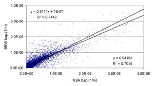
Fig. 3.4 Comparison of hourly-averaged absorption data from NSA and BRW.

For daily-averaged data (Figure 3.5), there is a stronger relationship between the two instruments’ measurements than for hourly averaged data and, again, good agreement for the two measurements of absorption coefficient. Because particle concentrations and hence, light absorption, are low at the site, often near the detection limits of the two instruments, there is considerable noise in the measurements. The improvement in fit for the daily averaged values with respect to the hourly averaged values is most likely a result of averaging noise in the data over a longer time period.

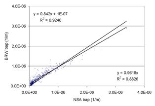
Fig. 3.5 Comparison of daily-averaged absorption data from NSA and BRW.

Figure 3.6 shows the variability in the ratio of the two instrument measurements as a function of absorption coefficient. The relationship between the two instruments appears less variable at higher absorption coefficients (s_ap > 1 Mm^-1) but only about 10% of the data are in this range. It is unfortunate that the polluted data are not recorded so that we could compare the instrument responses at higher particle concentrations. At low absorption values (s_ap < 1 Mm^-1) there is considerable variability due to instrument noise. Interestingly, while the aethalometer data are lower than PSAP data for high absorption coefficients (consistent with the linear fit results) the aethalometer measurements tend to be lower than the PSAP’s at low s_ap.

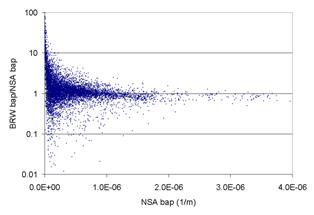
Fig. 3.6 Variation in the ratio of absorption measured at BRW to that measured at NSA as a function of absorption coefficient.

Table 3.6 summarizes the fit parameters for the absorption coefficient. Overall, the linear fits suggest that the BRW measurements were consistently lower than the NSA measurements. There are other questions which should be addressed with respect to measurements of s_ap at Barrow. These include: How much do the differences in wavelength of the two instruments influence s_ap? Is some of the variability in the two instruments due to differences in polluted sector data removal – does the NSA system the use same wind data as the BRW system? Are there corrections which should be applied to the aethalometer: for example some sort of spot size correction? How appropriate is the arbitrarily chosen 10 m²/g which used to convert from mass concentrations measured by the aethalometer into scattering coefficients?

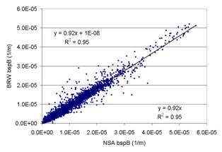
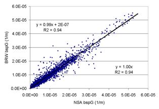
In addition to comparing absorption coefficient measurements, comparisons of scattering coefficient as a function of wavelength for the BRW and NSA nephelometers were also made for a one year period starting October, 1997. Table 3-7 summarizes results for the scattering coefficient comparison. For the two nephelometers there is high correlation, despite low particle concentrations and hence low scattering measurements. The blue scattering coefficients show the largest discrepancy. This may be due to problems with the blue photo-multiplier in the BRW nephelometer. The blue scattering measurement at BRW was often similar to or even lower than the green scattering measurement, while at NSA the s_spB /s_spG ratio was typically greater than 1 as expected (see Figure 3.7 a,b,c).

Differences between the two instruments may be attributable to several factors. Optically, the two nephelometers are (almost) identical, so it was assumed that correcting for truncation angle would not improve the comparison, thus for this comparison no corrections for truncation were applied to either instrument. Changes in filter bandpass and calibration error may also play a role.

b)

b)

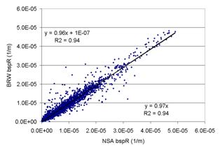
Fig. 3.7 Comparison of hourly averaged scattering coefficients measured at BRW and NSA for blue (450 nm) green (550 nm) and red (700 nm) wavelengths.

Optical Property of Indian Ocean Aerosols

During February and March of 1999 the CMDL aerosol group participated in the Indian Ocean Experiment (INDOEX), a multi-platform field campaign that took place over the Indian Ocean. A central focus of the campaign was to assess the role of aerosols from the Indian subcontinent on direct and indirect radiative forcing as well as the role of convective cirrus in aerosol transport and photochemical processing.

b)

This region of the world has a fast growing population that is becoming more industrialized with emissions of CO₂, aerosols and sulfates expected soon to surpass those of North America and Europe. Because of these potentially high future emissions, an understanding of climate forcing and transport of trace gases and aerosols in this region is critical to being able to predict global climate forcing.

c)

The INDOEX campaign was based at the Maldive Islands, which is about 700 km southwest of India. As part of the campaign NOAA/CMDL performed direct measurements of aerosol optical properties on two separate platforms; the U.C. San Diego - Scripps climate observatory on the island of Kaashidhoo (KCO) and on-board the NCAR C-130 aircraft. These measurements include the aerosol total and hemispheric backscattering coefficients, the aerosol hygroscopic growth factor (f(RH)), and the aerosol absorption coefficient. Here we define the aerosol hygroscopic growth factor to be the ratio of aerosol scattering coefficients at 85% relative humidity to aerosol scattering coefficient at 40% relative humidity.

Aerosol optical measurements operated at KCO from February 12 to March 28, 1999. During the northeast monsoon season (January-April) the Intertropical Convergence Zone is south of the island and air circulation is from the Indian subcontinent. Thus, aerosols measured at KCO during this time represent polluted continental air masses. Figure 3.8 shows a time series of the measured aerosol optical properties at KCO.

Back trajectory calculations show a change in the air mass origin on March 7^th (Day 66) from the east Bay of Bengal region to the west Arabian Sea. Evidence of this change is apparent in a decreased aerosol loading and accompanied by lower s_sp and s_ap values. Despite this difference in aerosol loading, the aerosol intensive properties of single-scattering albedo, backscatter fraction and hygroscopic growth are similar between the two regions. The lower aerosol loading in the Arabian Sea air masses likely resulted in a larger contribution to the total scattering from supermicron sea salt particles as evident in the smaller fractions of submicron aerosol scattering and absorption from the Arabian Sea.

Table 3.8 lists the mean values of the measured parameters and compares them to those from other CMDL surface sites. In comparison to aerosol properties measured at Bondville (a US continental site) and Sable Island (an Canadian marine site) the aerosol from the Indian subcontinent has a far greater absorption coefficient and lower single-scattering albedo. Unlike aerosols from U.S. continental sites, the single scattering albedo at KCO declines with an increase in aerosol loading (Figure 3.9). Apparently, under highly polluted conditions the aerosol soot fraction relative to sulfate is higher than that from US sites. This difference could reflect the regional sources of sulfate and carbon as well as rates of in-cloud sulfate oxidation. Although the Indian subcontinent aerosol has a large absorbing fraction, its mean hygroscopic growth is similar to that from regions with less absorbing aerosol. This difference points to either a significantly different composition or morphology for the absorbing components of aerosols from the Indian subcontinent with respect to North America.

Fig. 3.8 Time series of measurements from KCO a) aerosol total and submicron scattering and absorption b) aerosol total and submicron single scattering albedo c) aerosol total and submicron hygroscopic growth. Al,l values are reported for mid-visible (green) wavelengths.

Fig. 3.9 Aerosol single-scattering albedo plotted against scattering coefficient (hourly average data). Data are from the four CMDL North American monitoring stations (entire period of record) and the Kaashidhoo Island station in the Indian Ocean (February & March 1999).

In addition to surface-based measurements at KCO, aerosol optical properties were measured in situ from the NCAR C-130 research aircraft using an aircraft version of the ground-based CMDL aerosol measurement system. Aircraft measurements were necessary for information on spatial (i.e., horizontal and vertical) and temporal variability of aerosol optical properties. Vertical profiles and horizontal legs at altitude were conducted to characterize aerosol variability in the region, with coverage of much of the Indian Ocean Basin between 8° S and 17° N.

The measured aerosol light scattering coefficients over the northern Indian Ocean were typically several times those observed at perturbed continental sites in the U.S. The aerosol was also substantially darker than U.S. sites, with an average single-scattering albedo for all flights near 0.85. The highest aerosol concentrations were observed in the northern Indian Ocean (north of the Maldives). Typical aerosol optical depths in the region, calculated using aircraft aerosol optical property data, were in the 0.15-0.35 range for most days. Elevated aerosol layers, decoupled from the surface, were observed in over 1/3 of the vertical profiles. Figure 3.10 shows two vertical profiles, with one showing the elevated aerosol layer.

TABLE 3.5 Description of instrumentation at Barrow, Alaska

Instrument	Period of Operation	Station	Comments
MRI nephelometer.	1976- Fall, 1998	BRW	4 wavelength, no size cut
Magee Scientific Aethalometer	1988 – present	BRW	broadband, no size cut Specific absorption of 10 m²/g used to convert [BC] to _ap
TSI Nephelometer (Model# 3563)	Fall, 1997-present	NSA	3 wavelength, 1 and 10 mm size cut
Radiance Research Particle soot absorption photometer (PSAP)	Fall, 1997-present	NSA	565 nm wavelength,1 and 10 mm size cut

TABLE 3.6 Results from linear fits of data to equation: BRW = m*NSA for absorption coefficient

Parameter	Slope	R²	Number of points
s_ap (hourly)Year 1	0.92+ 0.01	0.66+ 0.01	3456
s_ap (hourly)Year 2	0.99+ 0.01	0.77+ 0.01	3562
s_ap (hourly)both years	0.94+ 0.01	0.70+ 0.01	7018
s_ap (daily)Year 1	0.94+ 0.03	0.88+ 0.02	223
s_ap (daily)Year 2	1.03+ 0.03	0.87+ 0.02	226
s_ap (daily) both years	0.96+ 0.02	0.89+ 0.01	449

Table 3.7 Results from linear fits of data to equation: BRW = m*NSA for scattering coefficient

Parameter	Slope	R²	Number of points
s_spB	0.92+ 0.00	0.95+ 0.01	3456
s_spG	1.00+ 0.00	0.94+ 0.01	3456
s_spR	0.97+ 0.00	0.94+ 0.01	3456

Table 3.8 Means and variabilities of pollution aerosols. Scattering coefficients, s_sp are for l = 550 nm. Absorption coefficients are at l = 565 nm. Fs_spG and Fs_ap are the submicron fractions of aerosol scattering and absorption, respectively. f(RH) is given for a relative humidity of 85% relative to 40%. Variabilities are reported as +/- one standard deviation. Sable Island, Nova Scotia and Bondville Illinois are anthropogenically perturbed marine and continental sites, respectively. The range of f(RH) at Sable Island is between polluted and clean air masses observed over a ~10 day period. Time periods of 4 hours before and after rain events were excluded from the KCO data.

Aerosol Property	Bay of Bengal	Arabian Sea	Sable Island	Bondville
s_sp	95+20	54+9	42+35	60+49
s_ap	25+7	10+3	2+2	5+4
F s_spG	0.70+0.06	0.62+0.05	0.26+0.10	0.86+0.07
F s_ap	0.85+0.04	0.80+0.07	0.81+0.10	0.82+0.10
f(RH)	1.65+0.10	1.67+0.14	1.7 + 2.7^*	1.5+0.4^**

*McInnes et al., 1998. **Koloutsou-Vakakis et al., 1999

Fig. 3.9. Two vertical profiles of aerosol optical properties obtained by CMDL instruments onboard the NCAR C-130 aircraft. Profile on the left shows a thick aerosol layer from the surface to ~2 km. Profile on the right shows an elevated aerosol layer with a peak at ~3 km altitude.

References

Barrie, L. A., Occurrence and trends of pollution in the Arctic troposphere, in Chemical Exchange Between the Atmosphere and Snow, Edited by E. W. Wolff and R. C. Bales, Springer-Verlag, Berlin, 1996.

Bergin, M.H., S.E. Schwartz, J.A. Ogren, and L.M. McInnes, Evaporation of ammonium nitrate aerosol in a heated nephelometer: Implications for field measurements, Environ. Sci. Technol., 31, 2878-2883, 1997.

Bergin, M.H., R.S. Halthorne, S.E. Schwartz, J.A. Ogren, and S. Nemesure, Comparison of aerosol column properties based on nephelometer and radiometer measurements at the SGP ARM site, J. Geophys. Res., 105,6807-6818, 2000.

Bergin, M.H., Meyerson, E., Dibb, J.E., Mayewski, P., Comparison of continuous aerosol measurements and ice core chemistry over a 10 year period at the South Pole, Geophys. Res. Lett., in press, 1998.

Bodhaine, B. A., Barrow surface aerosol: 1976-1987, Atmos. Environ., 23(11), 2357-2369, 1989.

Bodhaine, B. A., Aerosol absorption measurements at Barrow, Mauna Loa and South Pole, J. Geophys. Res., 100, 8967-8975, 1995.

Bodhaine, B. A., and E. G. Dutton, A long-term decrease in Arctic Haze at Barrow, Alaska, Geophys. Res. Lett., 20, 947-950, 1993.

Bodhaine, B. A. and J.J. DeLuisi, An aerosol climatology of Samoa, J. Atmos. Chem., 3, 107-122, 1985.

Bodhaine, B. A., J. J. DeLuisi, J. M. Harris, P. Houmere, and S. Bauman, Aerosol measurements at the South Pole, Tellus, 38B, 223-235, 1986.

Bodhaine, B. A., J.J. De Luisi, J. M. Harris, P. Houmere, and S. Bauman, PIXE analysis of South Pole aerosol, in Nuclear Instruments and Methods in Physics Research, B22, pp. 241-247, Elsevier, Holland, 1987.

Bodhaine, B.A., Harris, J.M., Ogren, J.A., Aerosol optical properties at Mauna Loa Obseratory: Long-range transport from Kuwait?, Geophys. Res. Lett., 19, 581, 1992.

Bond, T.C., T.L. Anderson and D. Campbell, Calibration and intercomparison of filter-based measurements of visible light absorption by aerosols, Aerosol Sci. Technol., 30, 582-600, 1999

Koloutsou-Vakakis, S., C.M. Carrico, M.J. Rood, Z. Li, R.Shrestha, J.A. Ogren, J.C. Chow, and J.G. Watson, Aerosol properties at a mid-latitude northern hemisphere continental site, submitted to J. Geophys. Res., 1999.

Charlson, R.J., S.E. Schwartz, J.M. Hales, R.D. Cess, J.A. Coakley, Jr., J.E. Hansen, and D.J. Hofmann, Climate forcing by anthropogenic aerosols, Science, 255, 423-430, 1992.

McInnes, L.M., Bergin, M.H., Ogren, J.A., Schwartz, S.E., Differences in hygroscopic growth between marine and anthropogenic aerosols, Geophys. Res. Lett., 25(4), 513-516, 1998.

NRC (National Research Council), Aerosol Radiative Forcing and Climatic Change, National Academy Press, Washington, D.C., 161 pp, 1996.

Ogren, J.A., "A systematic approach to in situ observations of aerosol properties", In Aerosol Forcing of Climate, edited by R.J. Charlson and J. Heintzenberg, John Wiley & Sons, Ltd., 215-226, 1995.

Quakenbush, T. K., and B. A. Bodhaine, Surface aerosols at the Barrow GMCC observatory: Data from 1976 through 1985, NOAA Data Rep. ERL ARL-10, 230 pp., NOAA Air Resources Laboratory, Silver Spring, MD, 1986.

Radke, L. F., C.A. Brock, R.J. Ferek, and D.J. Coffman, Summertime Arctic hazes, paper A52B-03 presented at the American Geophysical Union Fall Annual Meeting, San Francisco, December 3-7, 1990.