Atmospheric Remote Sensing: Instruments
FLOE Field Programs

Arctic Stratification
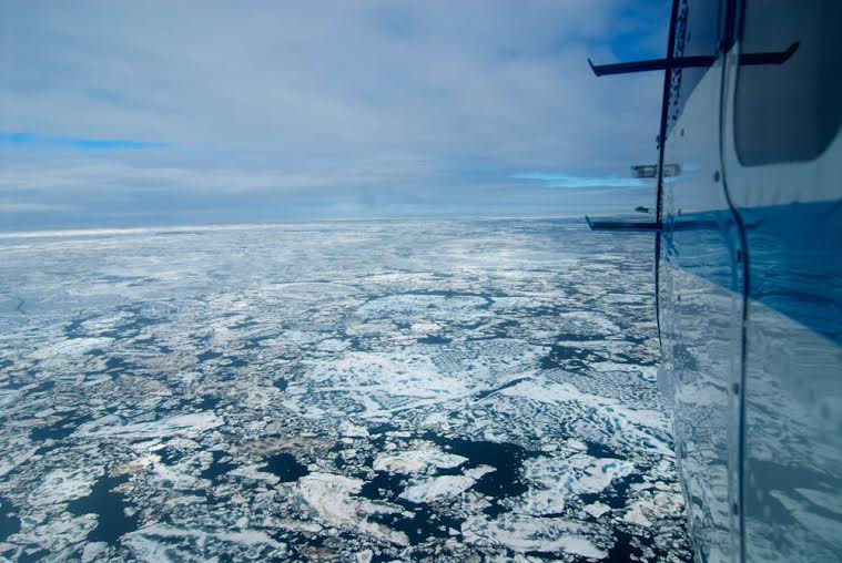
Three expeditions were made to the Alaskan Arctic to study the effects of retreating sea ice on phytoplankton distributions and primary productivity. These were in July of 2014 and 2017 and May of 2019. In July of 2014, the ice edge was roughly even with the northern tip of Alaska, the ice was retreating rapidly, and the phytoplankton was generally found in subsurface layers in open water and in the Marginal Ice Zone (Churnside and Marchbanks, 2015). In July of 2017, the ice was much farther north. It was still melting rapidly and the phytoplankton was still found in subsurface layers as in 2014 (Churnside, et al., 2020). In May of 2019, the ice edge was about where it was in July of 2017, much farther north than expected. While the ice edge was similar, the plankton distribution was very different. Instead of subsurface layers, it extended clear to the surface. It was stronger in open water than in the Marginal Ice Zone, but the vertical distribution was the same.
Gulf of Mexico
In late September and early October 2011, FLOE was installed on a small (King Air 90) twin-engine aircraft, deployed to Stennis International Airport, Mississippi. FLOE flew in coordination with the R/V McArthur II to survey epipelagic organisms (juvenile and adult small pelagic fish and gelatinous zooplankton) in the surface waters of the northern Gulf of Mexico (Churnside et al., 2017) potentially affected by the Deepwater Horizon oil spill and in surrounding areas. The oceanographic fish lidar was able to penetrate to > 30 m in offshore waters and 20 - 30 m on the shelf, except for the Mississippi River plume, where penetration was < 20 m. Few dense schools were detected, and those were generally found on the shelf. Several of these were positively identified as aggregations of moon jellies (Aurelia sp.). ( Churnside et al., 2016). Large numbers of flying fish were detected, especially off the shelf (Churnside et al., 2017). Generally, more schools and single targets were detected at night than during the day, suggesting diurnal migration. Other features, including large layers and plumes were also observed. The layers are probably phytoplankton, but some of the plume structures might be oil from seeps. Comparison with the data from the surface vessel will be used in the final analysis to confirm the identity of the features detected by FLOE.
We returned to the Gulf of Mexico in July, 2015 to measure the distribution of optical backscattering coefficient, bb. The lidar values were compared with in situ values measured from a Slocum glider. We found a moderate correlation (R = 0.28, p < 10-5), with differences that are partially explained by spatial and temporal sampling mismatches, variability in particle composition, and lidar retrieval errors (Churnside et al, 2017).
Lake Erie
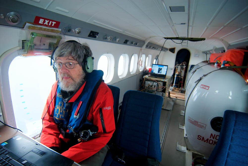
In August, 2014, the lidar was installed on a NASA Twin Otter for flights over the western basin of Lake Erie. This part of the lake is subject to toxic cyanobacteria blooms in summer. The vertical distribution of cyanobacteria is important, because the drinking water intakes for various municipalities are below the surface. Two species were present, Microcystis and Planktothrix. The first tends to form a dense mat at the surface, while the second is distributed deeper into the water column and is more of a threat to drinking water. The lidar was able to successfully measure the depth distribution of the bloom across the western basin of the lake (Moore, et al., 2019).
East Sound
In the spring and summer of 2009 - 2012, we took the lidar to East Sound, Orcas Island, Washington State. The sound is a well-known natural laboratory for the formation of thin plankton layers. Thin layers of phytoplankton may contain densities of organisms ranging up to 1000 times those found just above, or below the structure. These extraordinary concentrations of living material must have important implications for many aspects of marine ecology (e.g. phytoplankton growth dynamics, micro- and macrozooplankton grazing, behavior, life histories, predation, harmful algal blooms). For our purposes, a thin layer was defined as a layer in the data less than 3m thick. Because the sound was within the line of sight of a hotel balcony at the head of the sound, we were able to install the lidar on a small Cessna aircraft and control it from the hotel using an antenna mounted on the railing of the hotel room deck. It operated almost like a drone, with the aircraft movements either preprogrammed (pre-flight briefing) or controlled in real time via radio link to the pilot. In this manner, we were able to make lidar profiles with high horizontal resolution for comparison with in situ data (Lee et al., 2013) and to make detailed measurements of a non-linear internal wave (Churnside et al., 2012).


Chesapeake Bay
In the summers of 2006, 2007, and 2008, we flew the lidar and a video camera over Chesapeake Bay surveying the relative abundance of menhaden. The lidar was able to detect fish much deeper in the water, but the video had a much wider swath width (Churnside et al., 2011). As part of the lidar investigation, we measured the target strength of menhaden by comparison with standard calibration targets in a tank.


Columbia River Plume
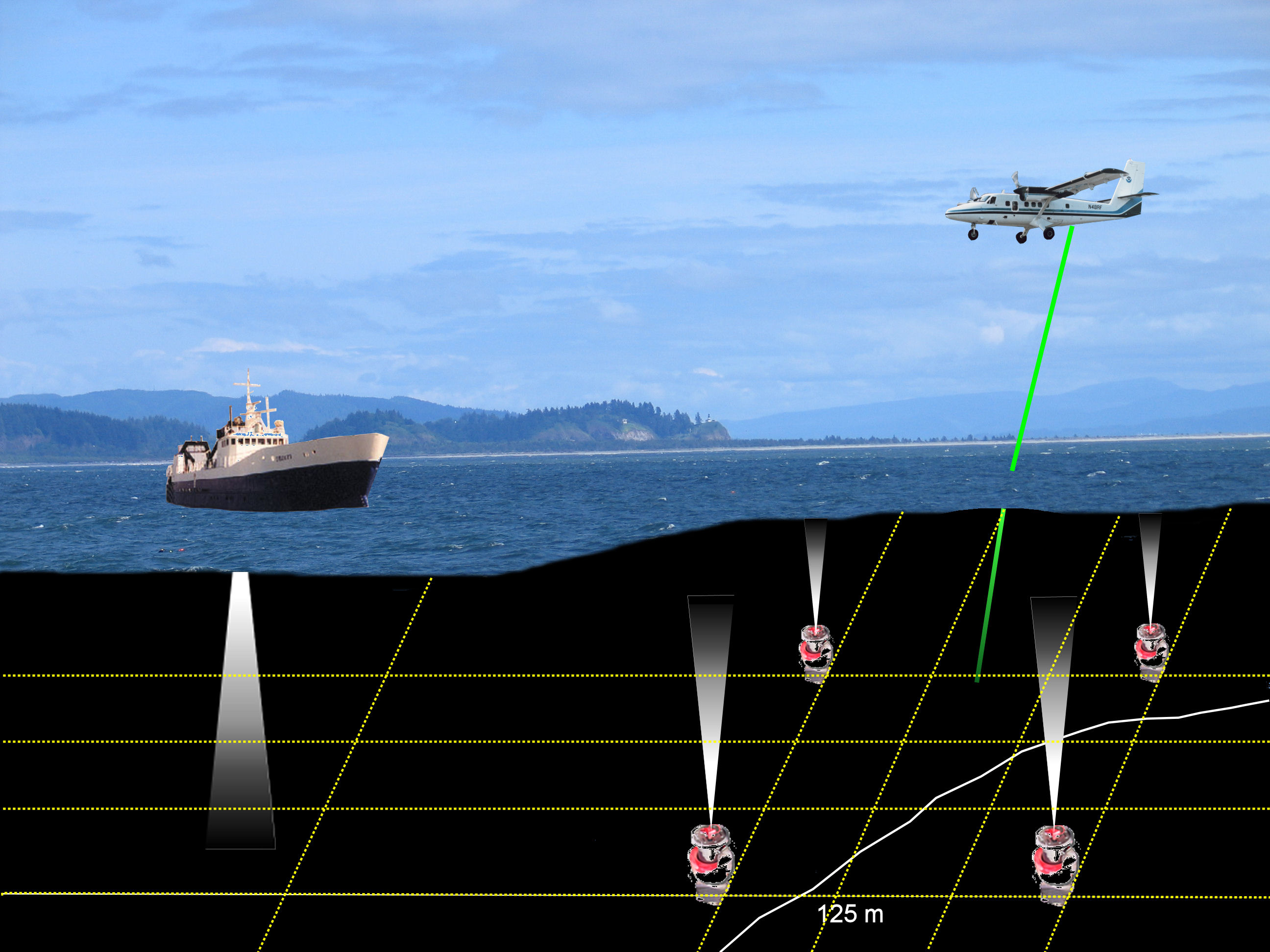
In 2003, 2005, and 2006, we flew the lidar off the coast of Oregon and Washington. The primary objective was to investigate the use of lidar, in conjunction with ship surveys and acoustic moorings, to measure the abundance of sardines (Churnside et al., 2009 ). We also documented the association of sardines with thermal fronts (Reese, et al., 2011). At the same time, the data were used to investigate the distribution of thin plankton layers in the Columbia River plume (Churnside and Donaghay, 2009). Finally, the data were used to describe two basic properties of lidar returns from the ocean. The first was the polarization characteristics, including the depolarization by multiple forward scattering (Churnside, 2008). The second was a study that documented the fractal nature of lidar scattering from the ocean, and measured the fractal dimension to be 1.76 (Churnside and Wilson, 2006).
Bering Sea
The lidar was one of a number of instruments studying survey strategies to assess Bering Sea forage species. Lack of information on forage species composition, distribution, and movements hinders our understanding of their ecological role in the Bering Sea. Recognizing the need for development of forage species survey strategies, this study characterized forage species in the slope, shelf, and nearshore regions of the Bering Sea using direct (midwater trawl, MultiNet, beach seine, jig, ROV) and indirect (acoustics, lidar) sampling technologies (Sigler et al., 2006 ). Forage species distribution and quantity differed between shelf (6-100 m) and slope (6-100 m, 100-300 m, 300 m-bottom) regions. Acoustics suggest that shallow and deep layers contained dispersed backscatter while the middle layer contained patchy schools. Lidar and visual measurements from aircraft documented a patchy distribution of surface plankton and densely shoaling fish that exhibited a high degree of temporal and spatial variability within the 10 d study period. In the nearshore, Pacific sand lance dominated catches and other commonly captured forage fish were young-of-year Pacific sandfish and gadids. Zooplankton density in the upper 100 m of the water column was significantly higher in nearshore waters. Though copepods were the most abundant taxa, euphausiids, second most abundant, provided more energy to predators due to their large size. We also documented an intense foraging event at a biological hot spot in the SE Bering Sea. This involved fish, whales, and sea birds all converging on a dense patch of euphausiids over the course of several days (Churnside et al, 2011).
Norwegian Sea
A broad-scale lidar survey was conducted in the Norwegian Sea in the summer of 2002 (Churnside et al., 2009). Since that survey, a number of data processing techniques have been developed, including manual identification of fish schools, multi-scale median filtering, and curve fitting of the lidar profiles. In the automated techniques, applying a threshold to the data has previously been shown to improve the correlation between lidar data and acoustic data. This is similar to applying a threshold to eliminate plankton scattering from acoustic data. We applied these techniques to the lidar data from the 2002 survey, and compared the results with the results of a mackerel survey performed by the ships FV Endre Dyrøy and FV Trønderbas during the same time period. Despite a high level of variability in both lidar and trawl data, we found that the broad-scale distribution of fish inferred from the lidar agreed reasonably well with the broad-scale distribution of mackerel caught by the FV Endre Dyrøy for manual processing of the lidar data and for manual processing of the lidar data using a median filter and a threshold level T > 1 . We also measured the optical target strength of Atlantic mackerel as a first step in a conversion to biomass (Churnside et al., 2006).
Gulf of Alaska
FLOE, along with a digital camera, was used in the waters off of southern Alaska in the summer of 2000 under funding from the North Pacific Marine Research Initiative. We evaluated airborne remote sensing, using lidar and color digital video, in the North Pacific in 2000. Specific objectives were (1) to determine lidar depth-penetration range, (2) to develop ocean color indices as a proxy for depth penetration and Chl a, (3) to compare lidar with acoustic and net-sampling data, (4) to define diurnal variability over large areas, and (5) to evaluate strengths and weaknesses. Depth penetration ranged from 18 to 50 m in non-silty water, with lowest values observed inshore by day and highest values on the continental shelf at night. A green index, derived from the three- band video data, was significantly related to depth penetration and was in general agreement with SeaWiFS satellite Chl a values. Significant correlations with acoustic data were obtained in an area with a high concentration of capelin, Mallotus villosus (Brown et al., 2002).
We returned in subsequent years in a collaboration with the Prince William Sound Science Center. We discovered a very high level of dissolved organic material in one of the inlets of Kodiak Island; the absorption increased dramatically in the inlet, without a corresponding increase in near-surface scattering. We demonstrated vessel avoidance by flying the lidar over one of the NOAA research vessels, the RV Miller Freeman. We demonstrated imaging of individual salmon using the laser as a light source for a gated intensified camera, which had an exposure time of 20 ns. (Churnside and Wilson, 2004). We demonstrated good agreement between lidar and echosounder measurements of zooplankton in Prince William Sound (Churnside et al., 2005).

Ghost Nets

Ghostnet refers to lost or abandoned fishing gear that drifts in the ocean continuing to catch fish and entangle marine mammals, turtles, and sea birds. The synthetic materials currently used in fishing nets decay extremely slowly, so these nets can continue to drift for years. Many of these end up trapped on the coral reefs, where entanglement rates are even higher than in the open ocean and where they damage the fragile coral. To remove these nets from reefs, divers must cut the nets off with knives and load them into inflatable boats. It is extremely laborious and dangerous work. During 2001, a multi-agency effort consisting of 3 ships and 18 divers removed nearly 70 tons of debris during 270 ship days at sea, clearing only two atolls in the 1200-mile Hawaiian Archipelago.
Given the magnitude of the problem and hazards associated with cleaning the reefs, a multi-agency effort is under way to locate ghostnets in the open ocean and collect them before they reach reefs. The ghostnet team has shown that many of these nets pass through the Sub-Tropical Convergence Zone north of the Hawaiian Islands in the spring of each year when the convergence is particularly strong. Oceanic debris of all types is expected to accumulate here and in other convergence zones. For this reason, searching for ghostnets and other debris in convergence zones was expected to be more efficient than searching the entire ocean. The effectiveness of this approach has been demonstrated in the North Pacific (Pichel et al., 2007).